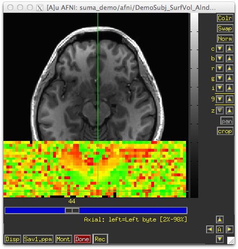
Press the t in the suma window to talk to afni. This sends
anatomically correct surfaces to AFNI.
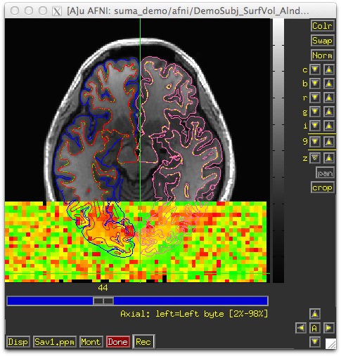
You should be seeing surface contours atop the slices; the contours
are the intersection of the surface with the slice.
AFNI slice view with anatomically correct surfaces
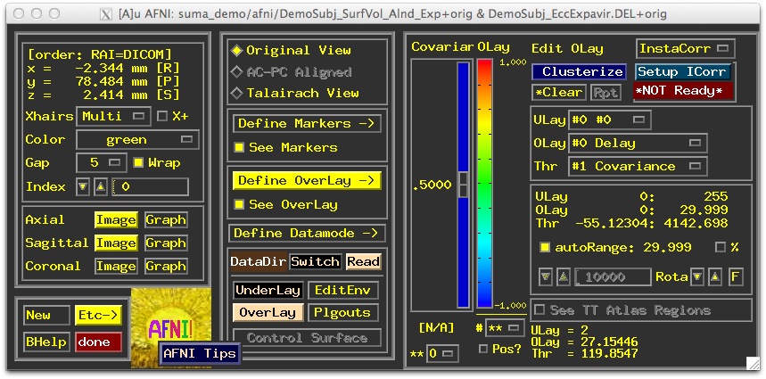
You should also see boxes representing the nodes that are within
+/-1/2 slice from the center of the slice in view. Colors and node
box visibility can be changed to suit your desires from the
ControlSurface button in AFNI.
Navigating through the volume in AFNI
Check to make sure you have an excellent alignment between volume
and surface. Also make sure surface adequately represents areas of
the brain that are difficult to segment:
occipital cortex
inferior frontal and inferior temporal regions
The surface may look good in suma, but it might not
actually match anatomy in some places – this is why you check
surfaces in the AFNI display.
The Surface Volume and the surfaces must be in nearly
perfect alignment.
If you have an improper alignment, it should be addressed here
and now. This should not happen for FreeSurfer and SureFit/Caret
surfaces created in the standard fashion with
@SUMA_Make_Spec_FS or @SUMA_Make_Spec_Caret,
say. Problems might come up when you attempt to align data
across days with @SUMA_AlignToExperiment. See also
Align_Surf_Vol
Watch for error messages and warnings to come up in the shell as
all the surfaces are read in. These messages should be examined
once per subject since they do not change unless the surface’s
geometry or topology is changed.
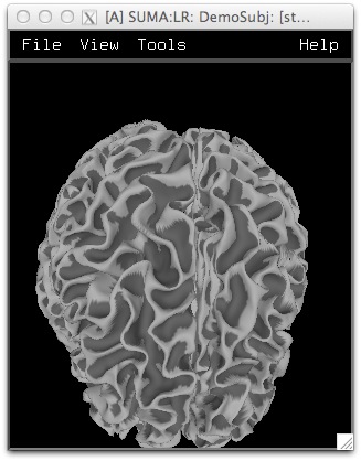
Viewed without the volume underal, it is extremely difficult to
tell if surface models with no topological defects accurately
represent the cortical surface.
Rotating the surface
Use Button 1 drag: keep it down while
moving the mouse left to right. This rotates the surface about the
screen’s Y-axis (dotted green if screen axes are
displayed). Let go of button-1 (usually the left button).
Repeat the left-click and drag, and move the mouse up and down in
order to rotate about the X-axis; and move the mouse in various
directions for rotations mimicking those of a trackball interface.
Arrow keys rotate by increments specified by the unix environment
variable SUMA_ArrowRotAngle in
degrees.
You can set SUMA environment variables in file ~/.sumarc. See
also option -update_env in suma.
Prying & Z rotating the hemispheres
Use Ctrl+button-1, drag: move the
mouse horizontally while button 1 is pressed and ctrl is down will
pry hemispheres apart for better visualization. The prying behavior
is different for spherical and flattened surfaces. Better try it
than read about it. See also F10
Use Shift+button-1 drag: Rotate
surfaces about screen’s Z-axis. This option is useful for
positioning flat surfaces when displayed one at a time. In most
other circumstances, it leads to confusion.
Press m to toggle momentum on. Click the left mouse
button and release it as you are dragging the mouse. It should
feel like you’re throwing the surface.
Lots more!
Function keys modify various aspects of the display
Those may be usurped by OS X, see Keyboard Setup or try key
modifiers to get them to work.
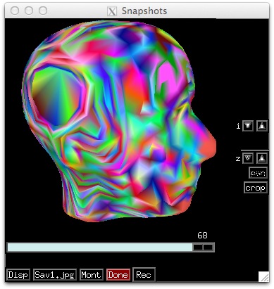
Press r in the viewer to record the current
scene. The image is captured in an AFNI flavored
window. Successive record commands get saved in the same viewer.
Note
The record viewer acquires a GUI interface the moment
it has more than one image in it. The interface is the
same as that in AFNI. If you want to save a single
captured image to disk, use ‘Alt+Right Click’ in the
recorder window to pop a save menu which allows you to
enter prefix of the image and more.
When more than one image are captured in the recorder,
you have numerous options to control the recording
process. Consider turning off
Disp->Save One to record multiple
images in one pass. This changes the save button from
Sav1.jpg to
Save.jpg. If you’ve read this far, you
should stop reading and try it for yourself.
Press r on the colorbar of the surface
controller records an image of the colorbar.
Press R to record continuously from the
viewer. Doing so puts the viewer in Recording Mode where
any operation that causes a change in the rendered image is
directly captured in the recorder.
Identical consecutive images are rejected
Images caused by window expose events are ignored
If you let the recorder run continuously with very large
images, you might quickly run out of memory on your computer.
Use Ctrl+r to capture the image directly to
disk intead of to the recorder.
From the available options, select one of
v2s.lh.TS.niml.dset, or v2s.rh.TS.niml.dset.
One of the two should be available to you depending on which
hemisphere is currently in focus. Contralateral dataset, if
sanely named, gets automatically loaded onto the contralateral
hemisphere.
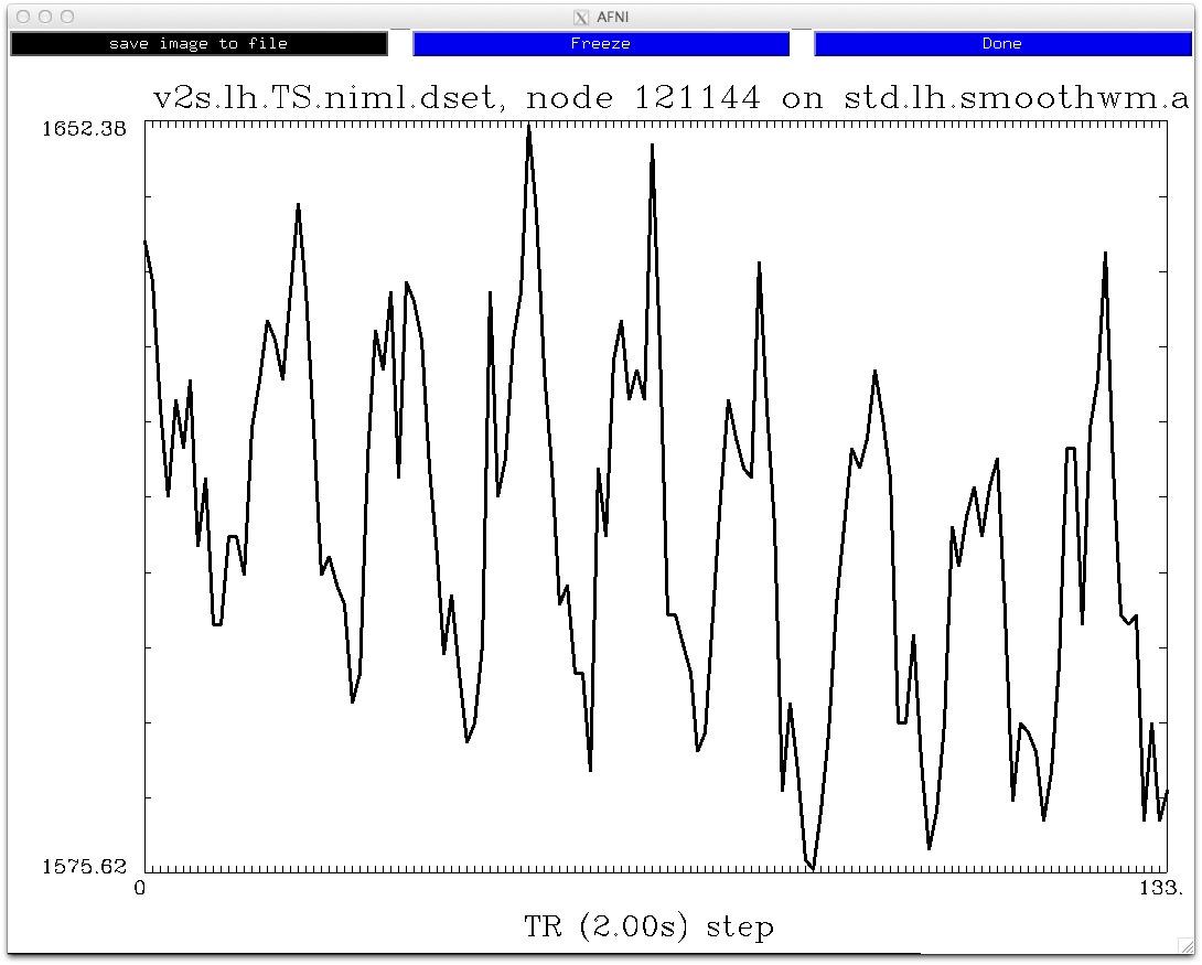
To graph the time series, at the cross hair press
g in SUMA. The graph window is wedded to the
hemisphere in focus. You will need to press g on
the contralateral hemisphere to get a graph for that hemisphere
too.
Press Freeze on graph window to preserve
current graph. Clicking on other nodes will start a new graph
For more help on graph window usage, including for instance
how to save the time series, type ctrl+h with the graphing
window in focus. (link)
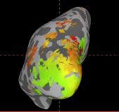
Now let’s look at a delay dataset (computed with
3ddelay). Press Load
Dset and load one of
v2s.lh.DEL.niml.dset or v2s.rh.DEL.niml.dset. SUMA
will colorize the loaded dataset thereby creating a color
plane for it, and will display it on the top of the
pre-existing color planes.
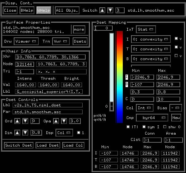
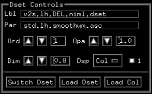
We begin by describing the right side block Dset
Mapping which is used to colorize a
dataset. Many of the options mimic those in AFNI’s Define
Overlay controls.
Note
Many features are not mentioned here, use
BHelp or WHelp interactively or the online help for
the controller you are using, here the surface
controller.
From the Dset Mapping block
on the right side of the interface
Use the scale to
set the threshold. Nodes whose cross correlation value does
not pass the threshold will not get colored.
Note p (uncorrected), and q values (FDR) below the
slider. FDR values are per-hemisphere
Note
For simplicity, we mapped a statistical dataset onto the
surface (see script run_3dVol2Surf under
suma_demo/afni). This resulted in
statistical parameters being averaged with being
normalized.
A better approach would be to map the time series, and
then perform the statistical computation. See script
run_3dVol2Surf for examples.
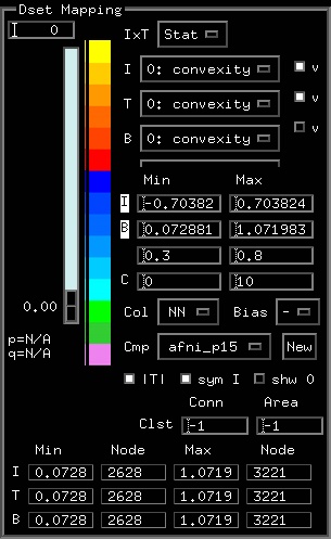
Mapping Parameters Table
This is located below the I, T, B selectors.
Used for setting the clipping ranges.
Clipping is only done for color mapping. Actual data values do
not change.
Note that a Left click on the
‘I’ locks ranges
from automatic resetting when you choose a different dataset column
for I. A right click on
‘I’ resets values
to full range in data.
For color mapping controls see
Col,
New,
Cmp, etc.
The colormap is rendered as a surface, and shares some of the
functions of SUMA’s viewer. You have keyboard controls when the
mouse is over the colorbar. More info
here and
there.
Interactive clustering
Left click on
Clst to
activate/deactivate clustering. Cluster table is output
to the shell. Clicking on a node shows its cluster label
in the viewer.
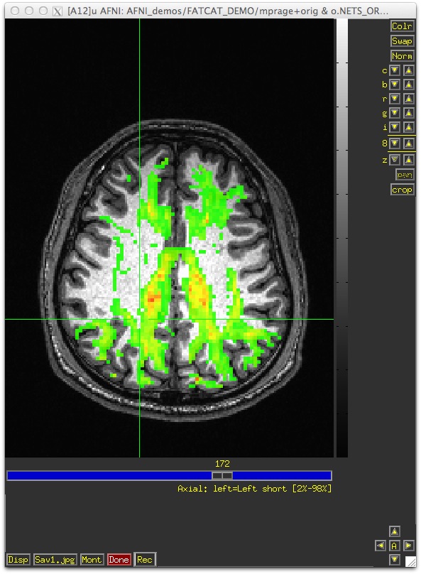
We present a brief example of viewing volumes in SUMA. This
particular case is one of looking at: probabilistic tractography
results (which are volumes), along with the target network that we
input (also volumes). We’ll load in the FA map from the DTI fits and
view it as slices for locating us in space. Finally, we can load in
the dset of structural connectivity for further information (labels,
graph connection and connectivity matrix viewing), but in this example
we won’t use it much, actually. Commands of note will be highlighted
with dashed ellipsoids (ell) for ease of finding.
To load in the appropriate data sets into suma, we use the
following commandline call from within the FATCAT_DEMO/DTI/
directory (assuming that you have run the scripts therein, you can
follow along at home). We are loading in most data as volumes (to
be viewed as either surfaces or slices), with the *.dset file
accompanying:
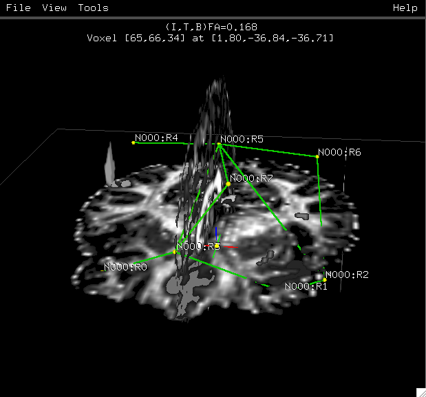
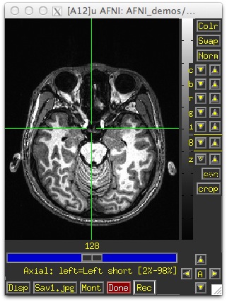
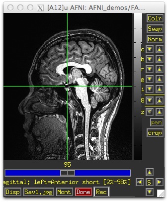
The following image is what we get (you may have different defaults
for some minor characteristics on your own machine, but this is
basically what should appear):
Volumes by default are viewed as slices, and in grayscale, so we
mostly see the FA map and not the PAIRMAP of tract results nor the
target ROI map. That default can be changed via environment
variable SUMA_VO_InitSlices in your
.sumarc file. If you have a volume rendered in 3D at this
stage, turn that off with the v
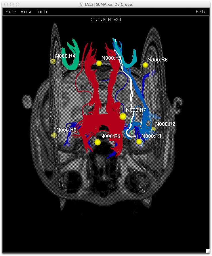
button. The dset is represented as a graph, showing the
centers-of-mass of the target ROIs with yellow spheres, and the
locations of tractographic bundles on lines, colored by a matrix
property in the dset.
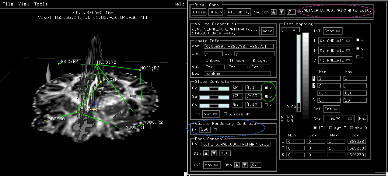
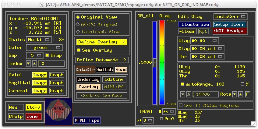
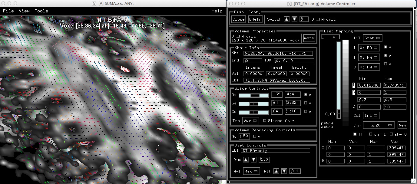
To really get going, let’s open up the controller, using either
“View -> Object Controller” or just the shortcut “CTRL + s” while
the SUMA viewer is foremost on the screen. Now we have the viewer
and the controller:
Each data object (here, volume or dset) will have its own control
panel, which we can toggle through using the small up/down triangle
“Switch” at the top of the panel (magenta ell.). But first, we
need to tell SUMA to prepare each panel, which we can most easily
do by hitting the “All Objs.” button (orange ell.). After this,
you can try toggling through each control panel, if you wish. (NB:
this useful button appeared in Jan, 2015, so if you don’t see,
please update your AFNI/SUMA distribution!)
Toggle to the PAIRMAP file using the switches at the top, seeing
the correct file name, in this case
o.NETS_AND_000_PAIRMAP+orig[0] (magenta ell):
This zeroth brick contains a mask of all the WM ROIs found between
any pair of targets in the image. Right now, it’s being shown as
slices, so it’s hard to appreciate. Let’s view these results as the
surface of the volume.
Firstly, turn off the slice viewing, by unchecking the slice
viewers, if they currently are highlighted (green ell.). Then,
turn on the surface viewing for the volume, by highlighting the
‘v’ in the “Volume Rendering Controls”
(blue ell). Additionally, in this same part of the panel, you can
adjust the density of surface rendering points, by changing the
number in the ‘Ns’ box; this parameter is now set to the maximum
number of slices in the volume. Increasing the number beyond this
value does not help much, decreasing the number speeds up the
rendering at the cost of more artifacts.
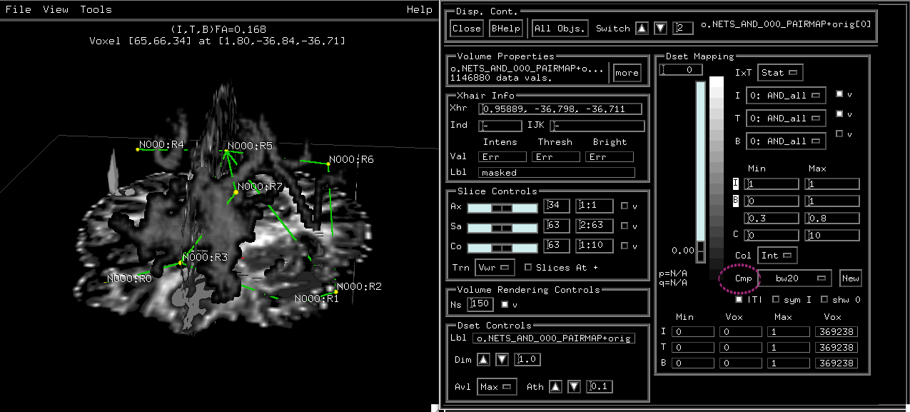
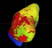
What you should see now is a big, gray mass of tract volume, as in
the SUMA Viewer window here:
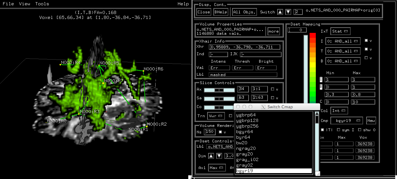
To change the colorscheme of the PAIRMAP (though, it is just a
binary mask in this case), we can go to the ‘Cmp’ button in the
Controller panel (magenta ell).
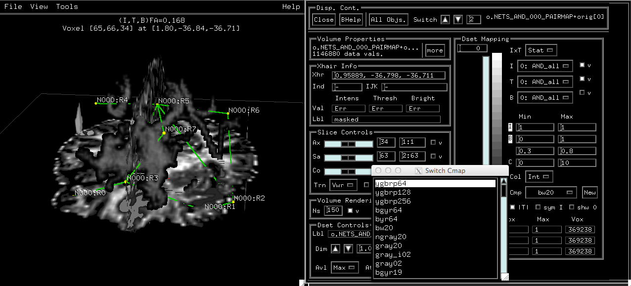
Right-click on the ‘Cmp’ button, which opens up a list of colormaps:
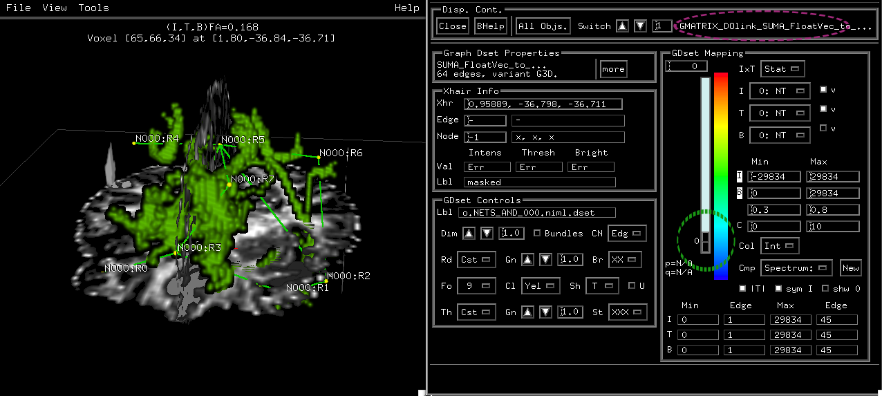
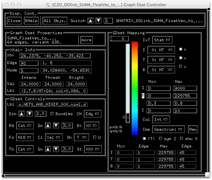
Now, let’s say we want to turn off the viewing of the dset data.
First, use the top arrows by the ‘Switch’ to go to the appropriate
Control panel, until you see something that says
“GMATRIX_DOlink…” at the top (magenta ell). NB for dsets: the
label here is not the filename in this case, but I think that what
is shown is a string inside the file– seeing ‘MATRIX’ should help
identify it:
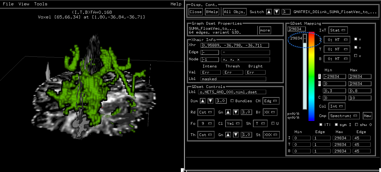
To not see any graph stuff, we’ll just raise the threshold for the
colorbar from ‘0’ (green ell) all the way to the top. Doing so
(blue ell in next figure), results in a farwell to labels and edges:
If you have no use for the dset at this time, you also didn’t have
to load it into the SUMA viewer, either.
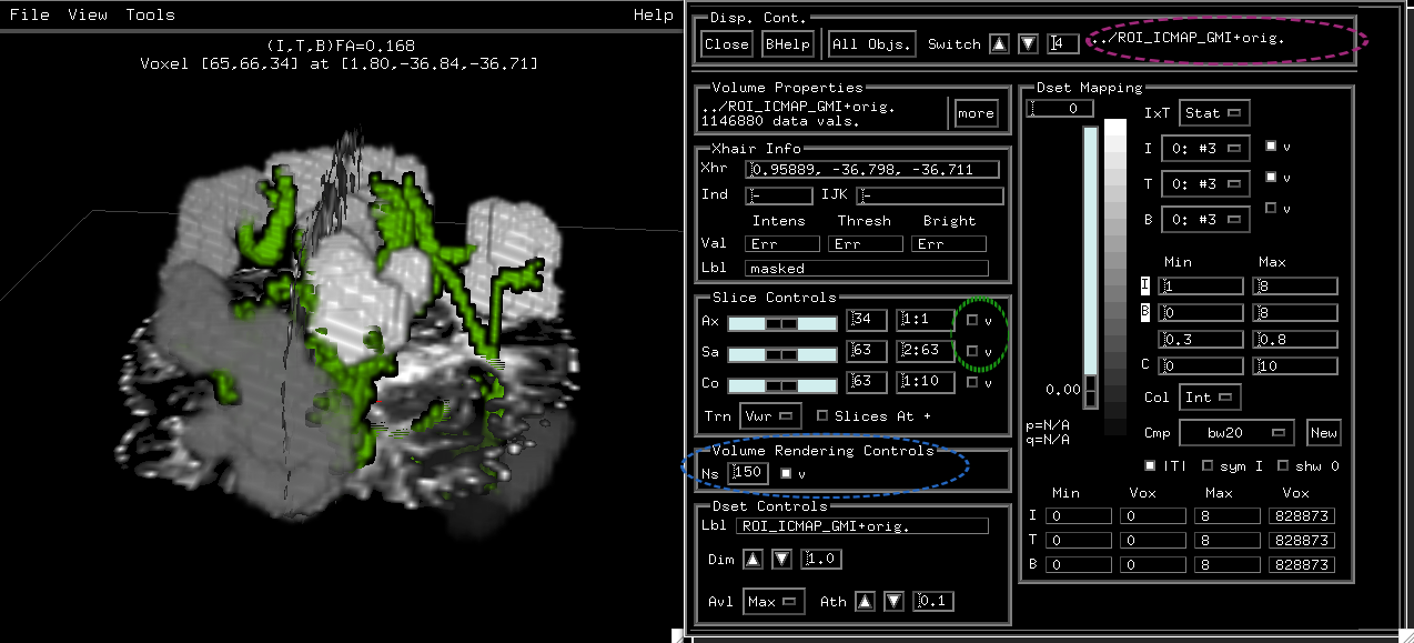
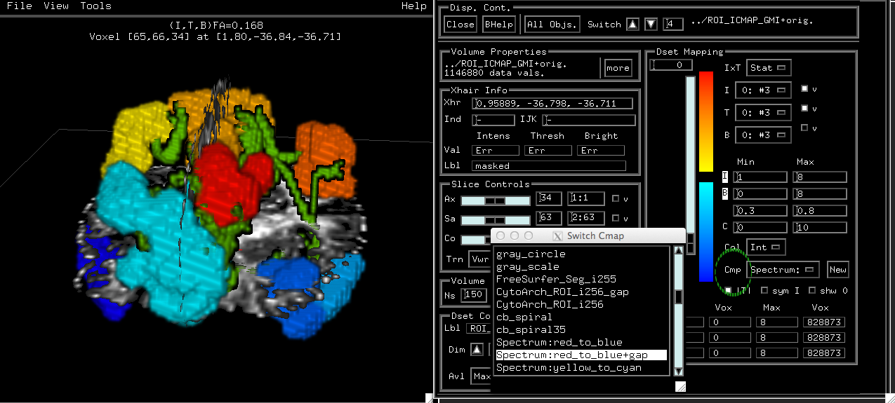
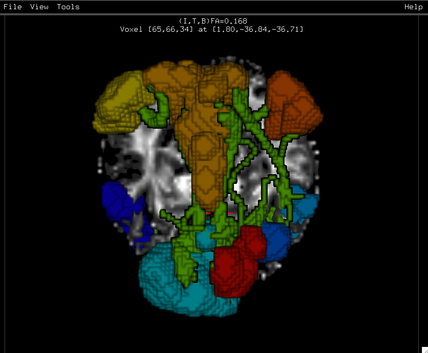
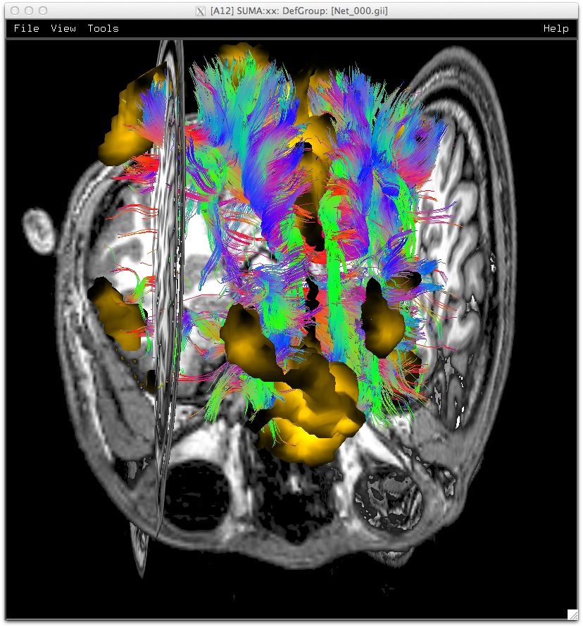
Ok, quickly now, let’s practice again by viewing the target ROI
network as surfaces. So, toggle to the panel with that volume’s
filename (here, “../ROI_ICMAP_GMI+orig”), and turn off the Slice
viewing and turn on the volume viewing, as done above, resulting
in a panel and viewer that look like the following (I’ve just
highlighted the locations from above where we had adjusted viewing
controls):
Again, we can make the volumes have a non-grayscale colormap for
viewing. In this case, each target ROI has a separate integer, so
a nice colorscheme could be the “ROI_i*” ones, or here I’ll pick
“Spectrum:red_to_blue+gap” from the ‘Cmp’ list (green ell in the
following) for no particular reason:
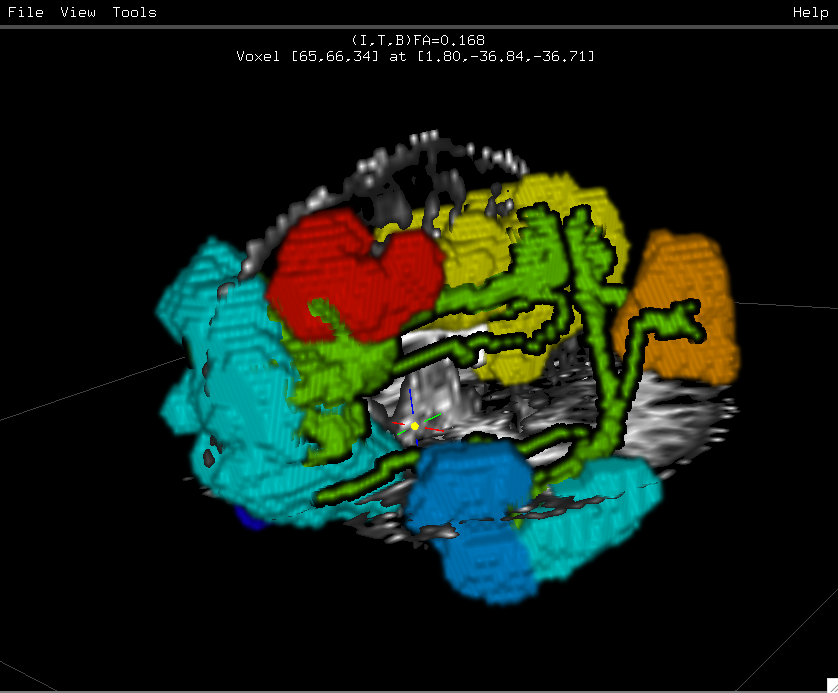
And that’s pretty much that! You can view the results from
different angles, and note that you can select voxels rendered in
3D much like you can select voxels on slices, tracts, etc.:
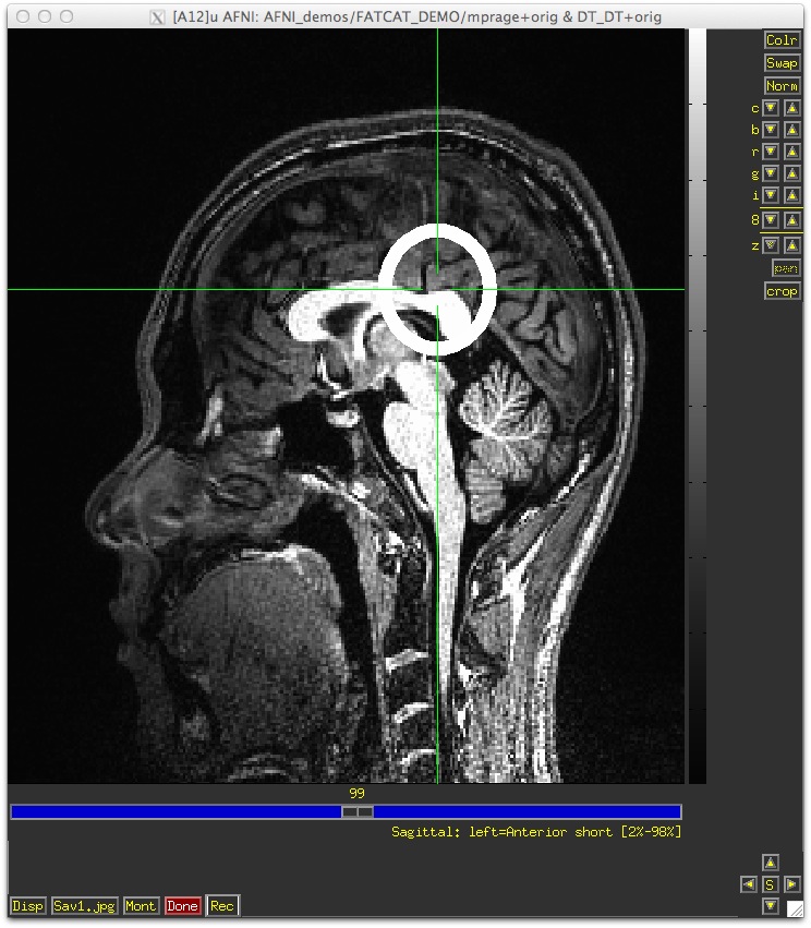
Right-click on the tracts to select a location along them. The
crosshair should mark the location along the tract where you
clicked. The selection would make AFNI jump to the same mm
location if the two programs are talking. To make them talk,
press t in the suma windowto get them talking and
try the selections again.
Left- middle-mouse buttons operate as they do for surface viewing.
Open the tract controller via
View‣ Object Controllers or
Ctrl+s. Select locations anew and examine
controller update coordinates and selection information.
InstaTract, or interactive mask selection
Create a mask by clicking on
Masks in the tract
controller. This creates a masking sphere and only tracts going
through it are displayed.
Selecting a location on the tracts will make the ball jump to
that location. Clicking on the slices or surfaces whenever
present, will position the mask at the selected voxel, or
surface node. If you select while dragging, the selection is
only made on the type of object on which you began the
selection. For instance, if you select a location on the tracts
and start dragging without releasing the right-mouse button, the
ball will track along non-masked tracts that fall under your
pointer, even if you go over surfaces or slices that are closer
to your viewpoint.
Tracts that fall outside of the mask are hidden by default. You
can also choose to display them in gray scale or in dimmed
colors by manipulating the hiding option.
To turn off ‘Mask Manipulation Mode’, right-double click in open air, or on the ball itself.
Another click on Masks will also open the masks
controller, which allows for complex masking
configurations. Check out the mask controller’s
link for information on how to manipluate the
mask in detail.
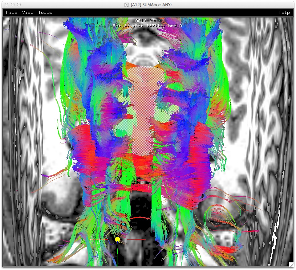
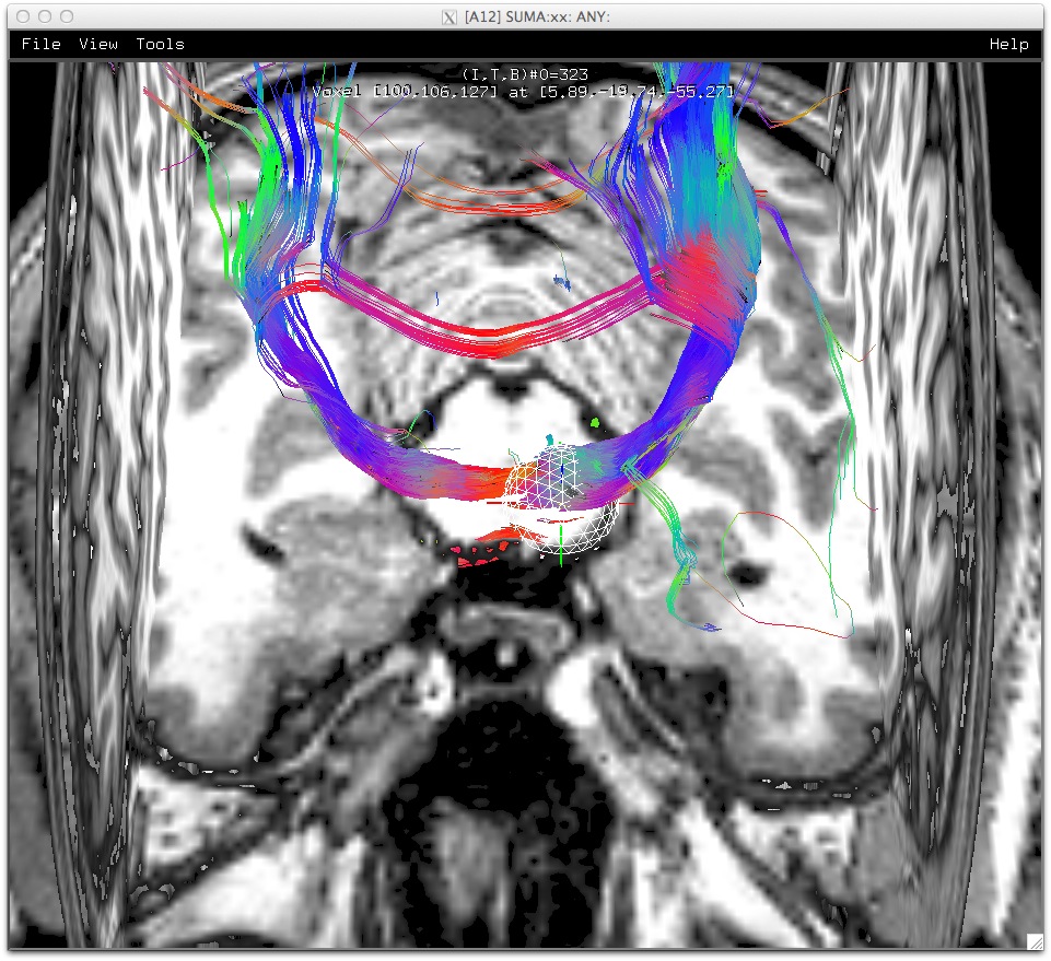
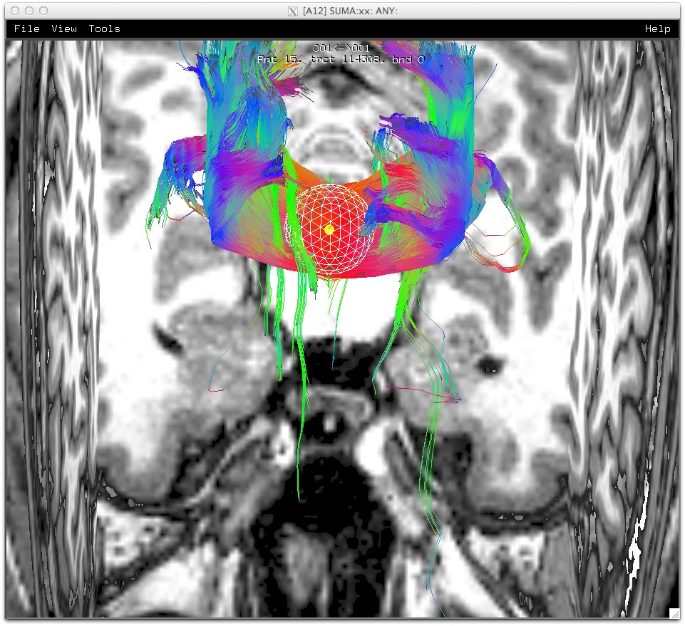
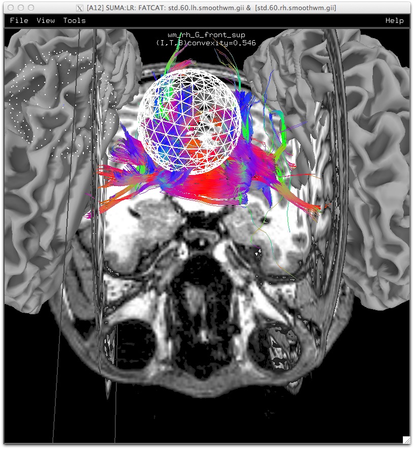
Looking at tracts within blobs making up one ROI
Here we are showing those tracts that go through any of the ROIs
in the DMN per the results of deterministic tracking in
3dTrackID that were generated in script
Do_05_RUNdti_DET_tracking.tcsh of
FATCAT_Demo.
This example is from the second part of demo script
Do_06_VISdti_SUMA_visual_ex1.tcsh. Close the old AFNI & SUMA
windows and launch new ones with the following commands:
The suma command now includes a set of surfaces
representing the ROIs. Those were created with program
IsoSurface in script
Do_05_RUNdti_DET_tracking.tcsh of
FATCAT_Demo.
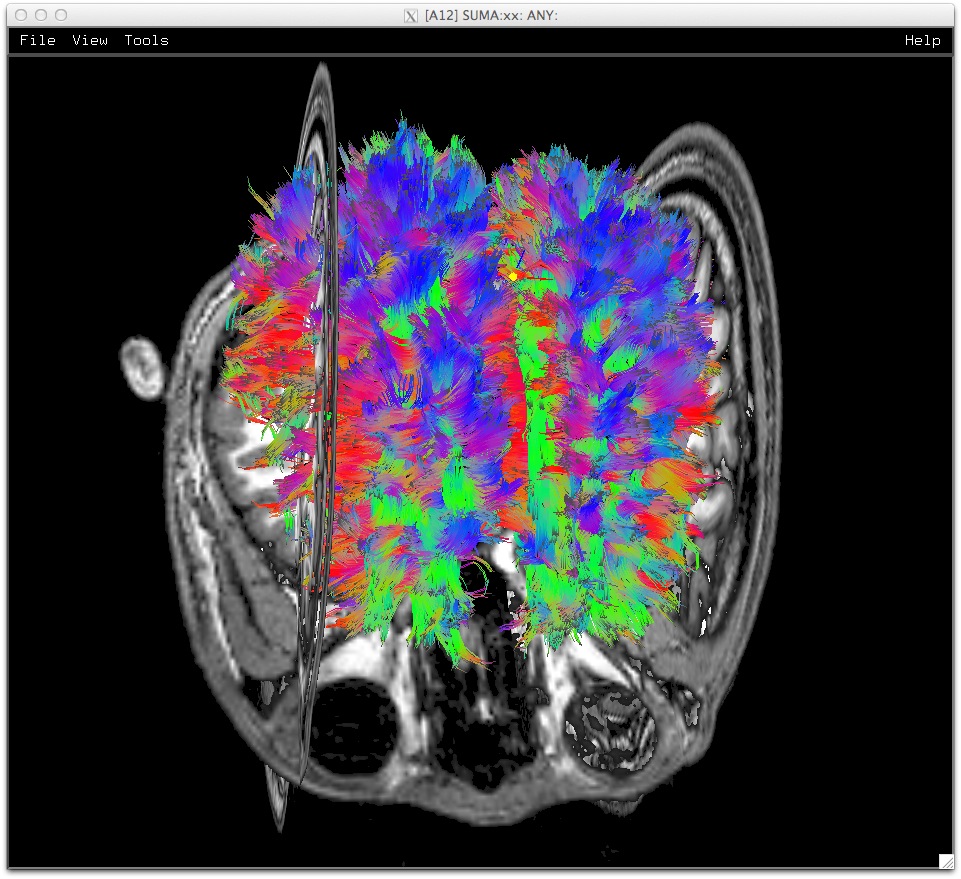
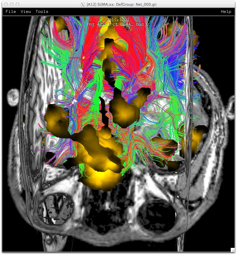
By default, points along the tracts are colored based on their
local orientation. You can also color them based on the
orientation of their midpoint with Switch Dset
‣ o.NETS_OR_000_MID accessible from the tract controller. You
can also color by bundle with Switch Dset ‣
o.NETS_OR_000_BUN, however there is only one bundle in
this set of tracts because there is only one ROI involved - all
the blobs are part of the same ROI in this example.
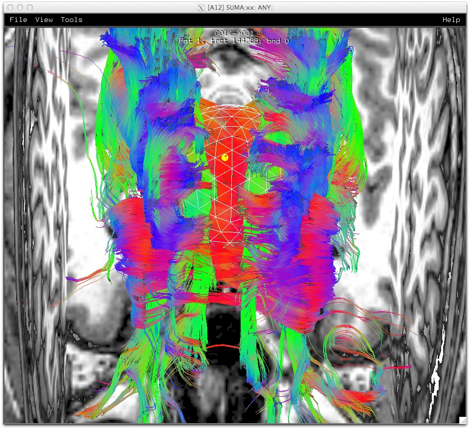
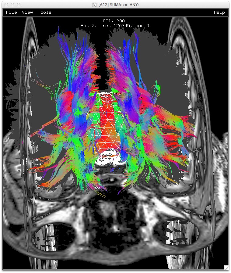
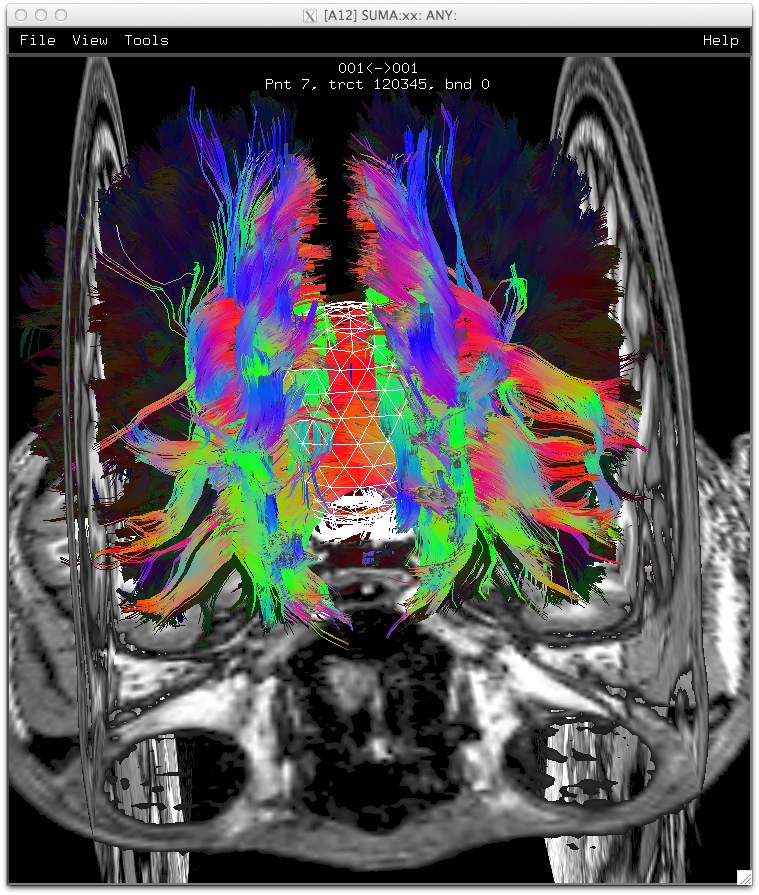
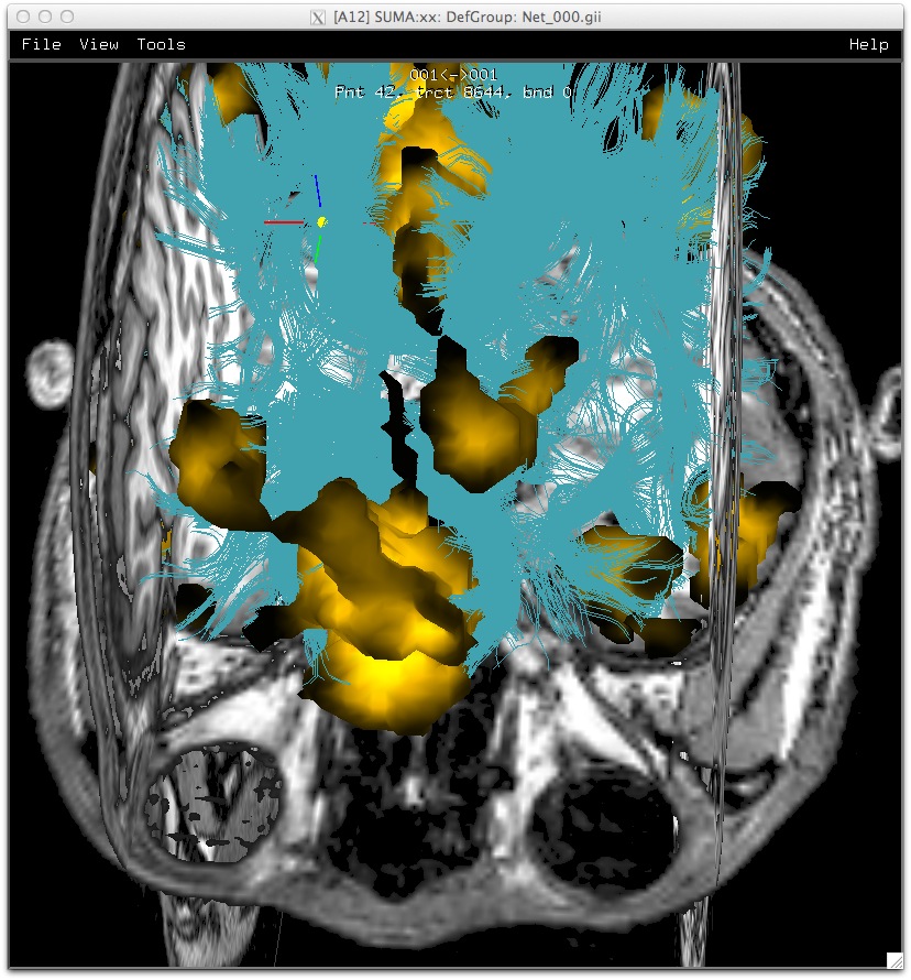
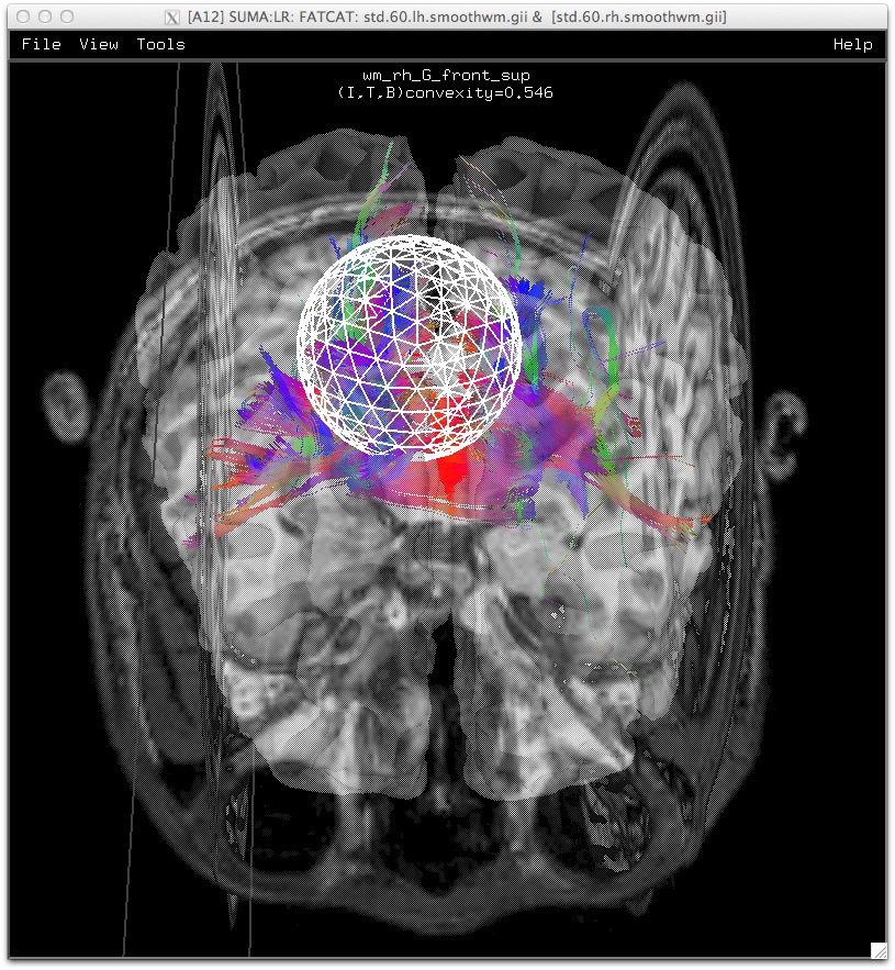
If you’re feeling adventurous, open the controllers for
the surface forming the ROIs by selecting a point on
the surface (the controller is created automatically once the
controller notebook is open), and
on a point of the volume to create the volume
controller. For the image blow, I hid the surface with
Drw, hid the
sagittal slice from the volume
controller, set the transparency to 8, then turned on the 3D
rendering with v.
This example is based on script
Do_09_VISdti_SUMA_visual_ex2.tcsh of
FATCAT_Demo. You can run it to launch the
demo automatically, or do it the hard way with:
The command uses the same data used in the Do_06 script, and in
paragraph 1 of the quick tour above, except
that we are also showing the cortical surfaces loaded via option
-spec.
Open the object controllers for volume,
tracts, and surfaces. Select
a tract and create a tract
mask. As mentioned
earlier, the mask can be positioned on the surfaces, just as you
would position it on the tracts or the slices. However the
surfaces obstruct the view and tracts are not visible. You could
make them transparent (press o twice in SUMA) but
that may not be ideal. Another option is to pry the surfaces
apart with ctrl+click and drag, left right, and/or up down. You
can now position the mask on the pried surfaces and have the
same masking effect. When the surfaces are pried apart, a
doppleganger of the mask is shown on the displaced surfaces, and
the mask ball is shown in the anatomically correct location.
Walk along the corpus callosum, for instance, and watch tracts
follow along. When talking to AFNI, correspondence between pried
surfaces and locations in the volume is maintained throughout.
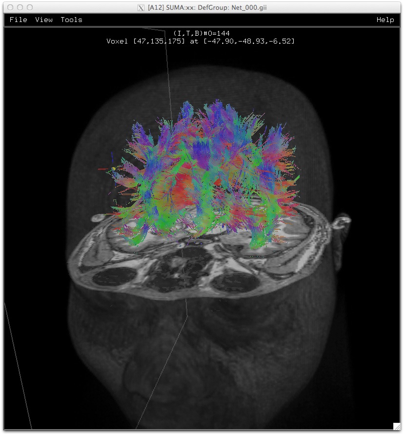
You can position the mask on the surface but few of the
tracts are visible this
way. (link)
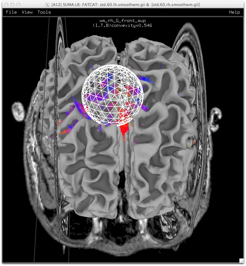
Surface pried open and viewer opacity turned off with two
more o. clicks
(link). You can continue
to position the mask on the pried surfaces.
Turning on 50% transparency for all objects by clicking
o twice - not thrice - helps, but not that cool
(link).
For more anatomical connectivity excitement, follow along with
remaining demos in script Do_09_VISdti_SUMA_visual_ex2.tcsh
and remaining Do_*VIS* scripts of
FATCAT_Demo.
This is a walk through the basics of graph (connectivity matrix)
navigation. To follow along you will need the FATCAT Visualization
directory installed.
For starters, we need to go into the demo directory and launch
suma and afni with the following commands:
The script Do_09_VISdti_SUMA_visual_ex2.tcsh contains the same
commands used above. New options to ponder for your amusement here
include -onestate, and
-gdset. Also, program
DriveSuma is used to control suma by mimicking
user input.For more driving good times, see also
@DO.examples, @DriveSuma,
and @DriveAfni.
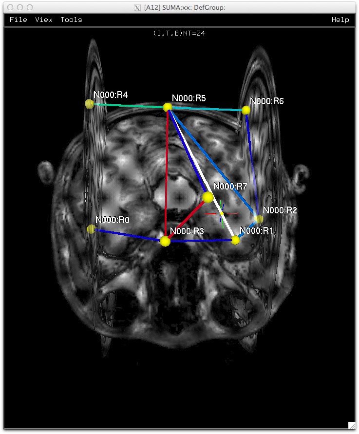
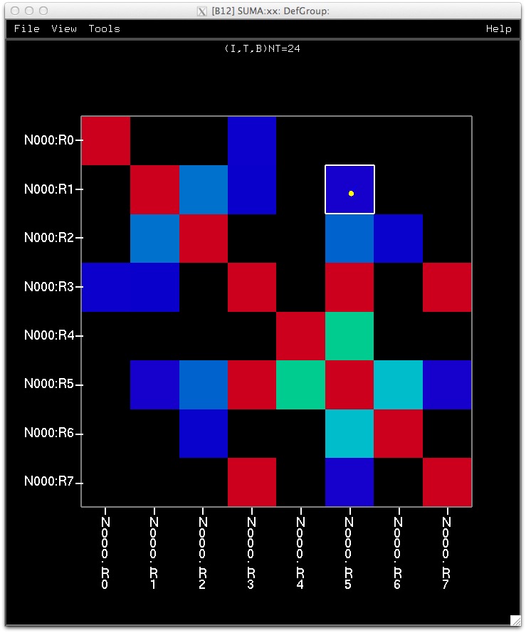
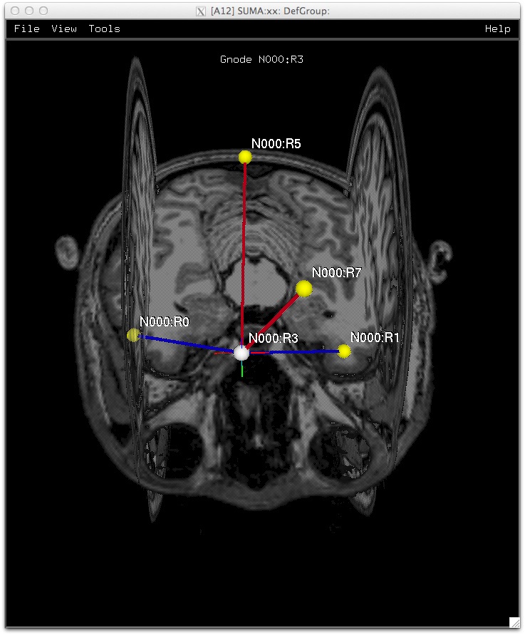
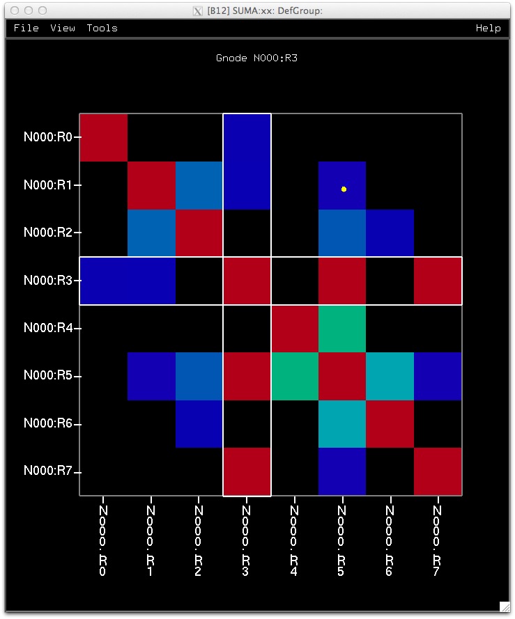
Let’s look at the connectivity matrices between DMN ROIs.
A connectivity matrix is considered a graph dataset in SUMA and can
be rendered as a set of nodes connected by edges, or as a
matrix. The dual forms can be rendered simultaneously this way:
The edges (cells) carry the connection values. Open the graph
controller with Ctrl+n to get
information about a particular connection, and do all the kinds of
colorization controls that are available for surface datasets and
volumes.
Selecting an edge highlights the cell in the matrix and vice versa.
Selecting a node (label, or ball in 3D graph mode, label in matrix
mode) will only show connections to that node.
The set of controls on the lower left side is particular to graph
datasets. Explore as curiosity moves you, the BHelp button comes in
handy here but the help messages are still a work in
progress. Complain away!
Of note is the Bundles
button, try it, it is cool.
Note that as with all AFNI datasets, you can have multiple
sub-bricks, here matrices of course. You can navigate
between them using the sub-brick selectors
(I,
T,
B) on the right side of the
controller.
So far, no thresholding was applied, so go ahead and try it out.
Show directions: for example, show surface based normals, explain
how you can hide some, etc. Link to other demos. For now, see
the following for some inspiration:
Interactive loading of displayable objects:
Ctrl+Alt+s
Demo script illustrating variety of DOs:
@DO.examples
D: Attch to the current dataset ‘parent’ a dot product
transform. The ‘child’ (transformed) dataset
is created by calculating the dot product between
each node time series and the time series of the current
node. Each time you ‘shift+ctrl+click (drag too if you like)’
on the surface, with the child dataset in view, the dot product
is recalculated.
You can save the resultant datasets with ‘ctrl+W’ key (see below).
Dset names are automatically formed.
To stop the interactive dot product computations,
switch back to the parent dset and press ‘D’ again.
If the parent dataset is properly detrended and each
time series is normalized so that its stdev is 1.0
then the dot product is the cross correlation coefficient.
Detrending and normalization can be carried out with:
3dDetrend -polort 4 -normalize
-prefix dt.TS.niml.dset v2s.TS.niml.dset
You can get a good feel for what this ‘D’ does by running
@Install_InstaCorr_Demo
That script will download and setup demo data for resting-state
correlations. In particular, script @RunSingleSurfInstaCorr of the
demo illustrates the ‘D’ feature.
Open a graphing window for the dataset
currently selected. The graphing window
updates with each new node selection.
A graphing window can be opened for each
dataset, and all graphs will update unless
‘1 Only’ is set in Surface Controller.
For complex data its magnitude is plotted instead.
Use ‘ctrl+h’ in graph window for more help.
in an a la AFNI image viewer.
Identical images are rejected.
If you just save one image, the recording
window has no visible controls for saving
the image. Either take another picture, or
use ‘Shift+right click’ to get a menu.
Images are saved with a date stamp of the
format PREFIX.X.yymmdd_hhmmss.MMM.jpg where:
PREFIX controlled with SUMA_AutoRecordPrefix.
See environment variable SUMA_AutoRecordPrefix for
controlling prefix and output image type (suma -update_env).
X The character indicating which viewer is recording (you can
record from multiple viewers at once.
yy, mm, dd, hh, mm, ss for year, month, day, hours, minutes,
and seconds, respectively. MMM is a millisecond marker to
avoid overwriting files. Unlike the other recording mode
(with the ‘R’ key), there is no rejection of identical images
This option is useful for saving a large number of images
without running out of memory in the recorder GUI.
Your current PREFIX is: ./SUMA_Recordings/autorecord.jpg
By increasing this factor, you can create
images at a resolution higher than that
of the SUMA window. This is done by subdividing
the scene into NxN sections and rendering each
section separately. The NxN renderings are
saved in the image recorder. After you
save the images to disk, you can stitch them
using imcat (a la AFNI montage).
Note that each section is still rendered at
the resolution of the SUMA window. So the bigger
the window the more resolution per section.
However, you cannot exceed a certain limit
on the number of pixels in the final image.
This limitation is due to the graphics card
on your system. SUMA will take care not to exceed
this limit.
Files are of 1D format with a necessary comment
at the top to indicate the type of objects in
the file.
Note 1: Repeatedly loading files with the same
name will replace currently loaded versions.
Note 2: Node-based (Types 3 and 4) objects
will follow a node when its coordinates change.
Note 3: See also ‘Alt+p’ for restricting which
node-based objects get displayed.
Type 1: Segments between (x0,y0,z0) and (x1,y1,z1)
1st line must be ‘#segments’ (without quotes),
or ‘#oriented_segments’ (slower to render).
One can also use #node-based_segments or
#node-based_oriented_segments and use a node index
in place of (x,y,z) triplets.
Remainder of file is N rows, each defining a
segment (or a vector) between two points.
Column content depends on the number of columns
in the file:
For node-based:
2 cols: n0 n1
3 cols: n0 n1 th
with th being line thickness
6 cols: n0 n1 c0 c1 c2 c3
with c0..3 being the RGBA values
between 0 and 1.0
Type 2: Directions, a variant of segments and oriented segments.
1st line must be ‘#directions’ (without quotes).
Remainder of file is N rows, each defining a
direction.
Column content depends on the number of columns
in the file:
3 cols: dx dy dz
with dx dy dz defining the direction. The
triplet need not be of unti norm though that
would affect the default coloring scheme detailed
below. The segment drawn has origin 0, 0, 0
4 cols: dx dy dz mag
with mag being a scaling factor for the direction.
mag is 1 by default.
5 cols: dx dy dz mag th
with th being the thickness of the line.
Default is 1
6 cols: ox oy oz dx dy dz
Specify the origin of the segment in o1, o2, o3.
Default is origin 0, 0, 0 for all
7 cols: o1 o2 o3 dx dy dz mag
Add individual scaling factors to case above
Segment is from origin to origin+mag*direction
8 cols: o1 o2 o3 dx dy dz mag th
Add thickness to case with 7 columns
9 cols: dx dy dz mag th c0 c1 c2 c3
Add colors for each segment, with origin at 0,0,0
11 cols: ox oy oz dx dy dz mag c0 c1 c2 c3
12 cols: ox oy oz dx dy dz mag th c0 c1 c2 c3
1st line must be ‘#spheres’ (without quotes).
Remainder of file is N rows, each defining a
sphere.
Column content depends on the number of columns
in the file:
3 cols: ox oy oz
4 cols: ox oy oz rd
with rd being the radius of the sphere
5 cols: ox oy oz rd st
with st being the style of the sphere’s
rendering. Choose from:
0: points
1: Lines
2: Filled
7 cols: ox oy oz c0 c1 c2 c3
with c0..3 being the RGBA values
between 0 and 1.0
8 cols: ox oy oz c0 c1 c2 c3 rd
9 cols: ox oy oz c0 c1 c2 c3 rd st
1st line must be ‘#points’ (without quotes).
Remainder of file is N rows, each defining a
point.
Column content depends on the number of columns
in the file:
3 cols: ox oy oz
4 cols: ox oy oz sz
with sz being the size of the point
7 cols: ox oy oz c0 c1 c2 c3
with c0..3 being the RGBA values
between 0 and 1.0
1st line must be ‘#node-based_vectors’ (without quotes)
or ‘#node-based_ball-vectors’ (slower to render).
Remainder of file is N rows, each defining a
a vector at a particular node of the current surface.
Column content depends on the number of columns
in the file:
3 cols: vx, vy, vz
node index ‘n’ is implicit equal to row index.
Vector ‘v’ is from coordinates of node ‘n’ to
coordinates of node ‘n’ + ‘v’
4 cols: n, vx, vy, vz
Here the node index ‘n’ is explicit. You can
have multiple vectors per node, one on
each row.
5 cols: n, vx, vy, vz, gn
with gn being a vector gain factor
8 cols: n, vx, vy, vz, c0 c1 c2 c3
with with c0..3 being the RGBA values
between 0 and 1.0
9 cols: n, vx, vy, vz, c0 c1 c2 c3 gn
Type 6: Spheres centered at nodes n of the current surface
1st line must be ‘#node-based_spheres’ (without quotes).
Remainder of file is N rows, each defining a
sphere.
Column content depends on the number of columns
in the file, see Type 2 for more details:
1 cols: n
2 cols: n rd
3 cols: n rd st
5 cols: n c0 c1 c2 c3
6 cols: n c0 c1 c2 c3 rd
7 cols: n c0 c1 c2 c3 rd st
Type 7: Planes defined with: ax + by + cz + d = 0.
1st line must be ‘#planes’ (without quotes).
Remainder of file is N rows, each defining a
plane.
Column content depends on the number of columns
in the file:
7 cols: a b c d cx cy cz
with the plane’s equation being:
ax + by + cz + d = 0
cx,cy,cz is the center of the plane’s
representation.
Yes, d is not of much use here.
There are no node-based planes at the moment.
They are a little inefficient to reproduce with
each redraw. Complain if you need them.
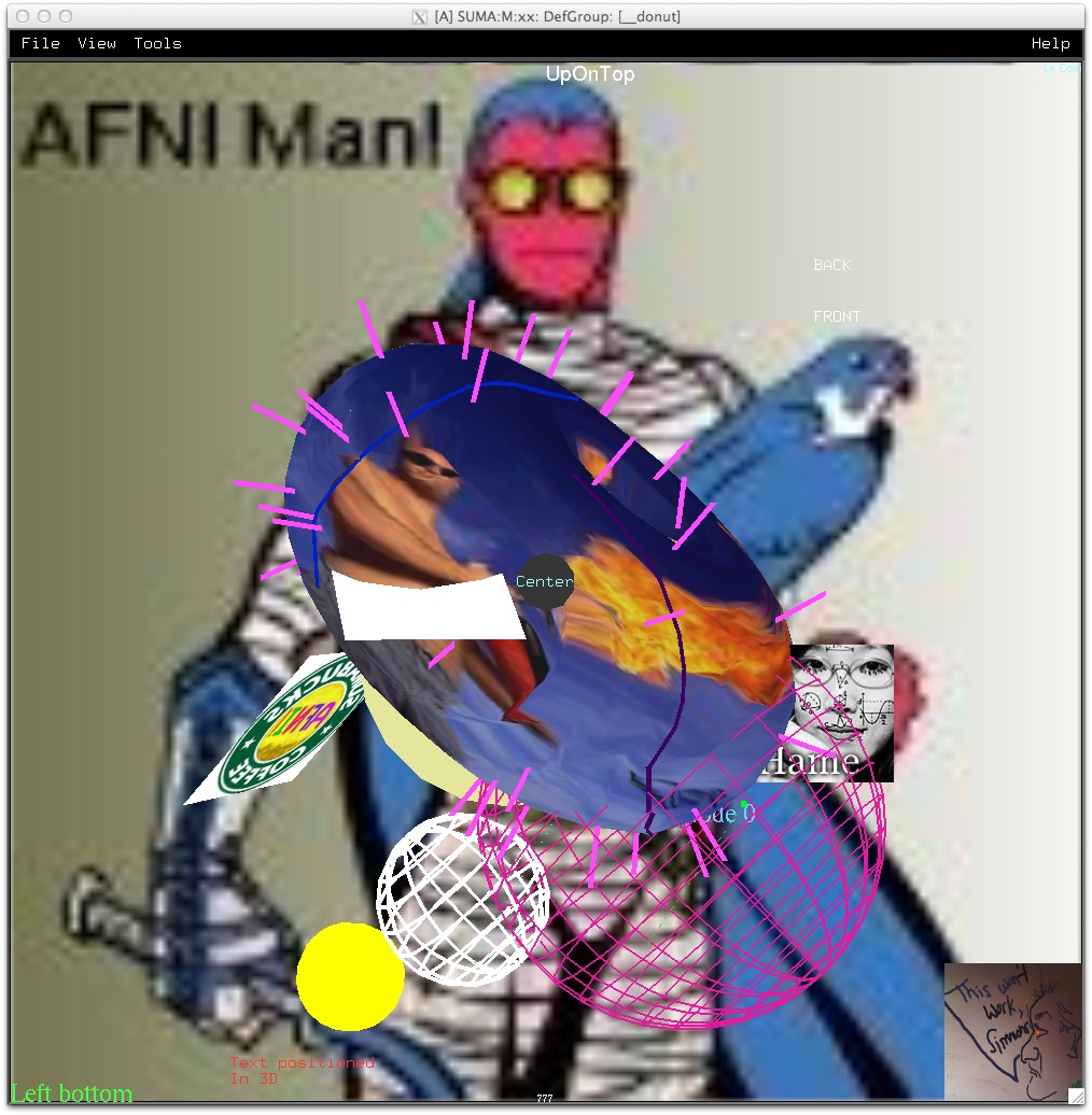
Type 8: Another class of displayble objects is described in
the output of suma -help_nido and the demonstration
script @DO.examples. This new class allows for displaying
text and figures in both screen and world space.
This is used to write temporary dsets that
are created on the fly in SUMA. Such sets include
those created via the ‘D’ option above,
or the results sent by 3dGroupInCorr
in the direction of the screen’s
X axis. The default is to move one
node at a time. You can alter this
setting with the environment variable:
SUMA_KeyNodeJump in your ~/.sumarc file.
This order will affect the resultant image in
the few instances where alpha transparency is
used. The order can be specified for only three types of
objects for now: graphs, surfaces, and volumes.
If you want to render graphs first, followed by volumes then
surfaces then set SUMA_ObjectDisplayOrder to something like:
‘graph,vol,surf’, or ‘GVS’
so that you can see medial or lateral walls better
from one angle. Prying is disabled for flat surfaces
and with spheres the effect is to rotate each sphere
about the Y axis passing through its center. Also, prying
is only enabled when the state you are viewing contains two
surfaces, one on the left and one on the right.
in 3D views, left right mouse movement cause a rotation about
the front or rear I/S axis.
Up down movements cause a shift along the left/right direction.
You can select nodes (Button 3) on pried surfaces and still
have AFNI jump to the proper location, and vice versa. However
for the moment, you cannot draw in pried mode. If you attempt
to draw, the surfaces are put back together.
To make best use of this option, you want to have env. variable
SUMA_LHunify = YES (see your ~/.sumarc for help)
In ROI mode, initiates a path to new node in DrawROI mode.
Picking of graph edges/nodes can get difficut
when surfaces are also displayed. To help with that,
see Alt+Button 3-Press next.
pick buffer. This is mostly for debugging or
for understanding why selection is behaving
strangely.
Shift+Button 3-Press: Shows an image of the selection buffer for debugging purposes. In Draw ROI Mode, the selection buffer is not displayed and the effect of the click is to select a node, but not to include it in the ROI.
the tract mask and turn the viewer into Mask
Manipulation Mode. In this mode, the mask is
shown as a wiremesh, and selections on any
object will move the mask to that location.
New tract/masks intersections are computed
at the new location.
To leave Mask Manipulation Mode, double
click with button 3 either on the mask or
in an area void of any objects.
If double clicking with a graph object in
focus and only connections from one node
are shown, then revert to showing all graph
connections. Without this, you can loose all
other clickables if a certain node is not
connected to anything.
Button 3-Motion: continuous picking whenever surface are present.
No calls for dot product (InstaCorr)
or GroupInCorr, while dragging.
Continuous picking of graph edges/nodes if no
surfaces are displayed.
The selection of an object triggers a multitude of actions:
When talking to AFNI, a selection prompts AFNI to also jump to the corresponding location. SUMA can also talk to other programs such asHalloSuma
The controller for that object is popped to the top of the stack in the controllers notebook, and the crosshair information in the controller gets updated.
Other open SUMA controllers are made to jump to the corresponding locations. Use the SUMA controller (Ctrl+u) to setup how different controllers are locked together.
When in drawing ROIs mode a selection adds to the ROI being drawn. See Drawing ROIs for details, assuming it is written by now!
If you have ‘click callbacks’ initiated, a selection combined with the proper keyboard modifiers initiates a callback. An example of this would be the surface-based instacorr or the variety of instacorr features in AFNI and/or 3dGroupInCorr. The following command can download and install demo material for InstaCorr excitement:
@Install_InstaCorr_Demo -mini
If you are in Mask Manipulation Mode Selections will make the tract mask jump to the selection location.
Picking behavior depends on the object being selected as follows:
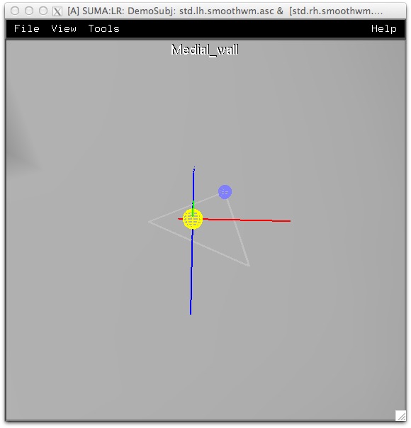
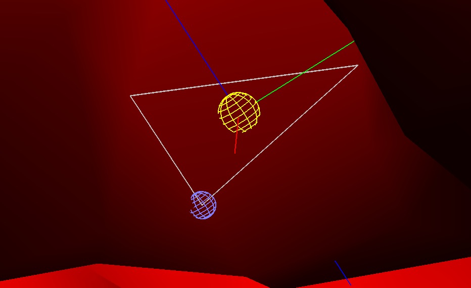
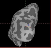
1- Node picking on surfaces: Selection of a node on the surface involves finding intersected triangles, identifying the closest intersected triangle, and then indentifying the closest node within it. The crosshair is centered at the location of intersection and marked with a yellow sphere. The closest node in the triangle is marked with a small (tiny some say) blue sphere, and the triangle is highlighted with a gray line contour. Highlighting can be toggled with F3 for crosshair, F4 for selected node, and F5 for the triangle
2- Voxel picking in volumes: You can select voxels on rendered slices as long as the voxels are not thresholded out of view. They maybe too dark to see but still be selectable if their value exceeds that of the threshold.
Selecting a voxel also highlights the slice. You can turn off the highlight rectangle with F5.
Note that you can also select from the 3D rendered volume and when 3D rendering is turned on. In that case, no slice highlighting is done.
3- Edge/cell selection in graphs: Right click on an edge, matrix cell, or bundle reprenting the edge and the connection is rendered white. Because the graphs can be bidirectional, clicking on an edge between [n1, n2] with the click location closest to n1 would select edge n1–>n2, while clicking closer to n2 gets you edge n2–>n1. This also happens when you click on a bundle representation of the edge. The selected connection is highlighted in white and the highlighting can be toggled with the F4
Selecting an edge on the 3D graph is reflected on the dual representation in matrix form by highlighting the equivalent cell, and vice versa.
Selecting a node on the 3D graph, by clicking on the ball representing the node, or the node’s name highlights only the connections to that node. The same type of selection can be made by clicking on a row or column’s label in the matrix representation form.
When graphs are represented along with volumes and surfaces, picking an edge can get tricky. In that case, use Alt+Button 3 instead.
4- Tract selection: Right click on a tract - the hairline - for selecting a location along the tract. What’s more to say ?
You can select and drag and sweep through numerous locations. The main thing to keep in mind is that when you have a multitute of object types, such as tracts, voxels, surfaces, etc. SUMA locks the selection to the object type selected at the beginning of the sweep. So, if you begin the selection on a surface and drag, then the selections during the sweep are restricted to surfaces only.
Increase is done by taking multiple shots that once stitched
together form a high-resolution image.
The maximum resolution is set by the GL_MAX_VIEWPORT_DIMS of your
graphics card. I have 4096 pixels.
If you exceed this number, SUMA will make adjustments automatically.
Assemble images with program imcat.
SUMA_NodeCoordsUnits (env): Coordinate units of surface nodes. Choose from ‘mm’ or ‘cm’
A bad choice can make the surfaces render with many artifacts.
default value: SUMA_NodeCoordsUnits = mm
SUMA_DoNotSendStates (env): Which anatomically correct surf. states should not NOT be sent to AFNI?
This is mostly for deciding whether one of ‘white’ or ‘smoothwm’
FreeSurfer states should not be sent to AFNI.
The default is to let them all go.
You can specify multiple states with a , delimited list (no spaces!).
By default nothing is excluded.
default value: SUMA_DoNotSendStates = N/A
SUMA_AutoRecordPrefix (env): Prefix for autorecord (suma’s Ctrl+R) files.
FreeSurfer states should not be sent to AFNI.
Add a path if you want the files to endup in a particular directory.
You can also add an extension to prefix to specify the output type.
Choose from .jpg, .ppm, or .1D . The fallback type is .jpg
SUMA_VO_Reorient (env): Force reorienting of read volume.
To force reorientation,
Choose from RAI, LPI, RAS. etc…
Use NO to avoid reorientation. This env. is for debugging purposes.
default value: SUMA_VO_Reorient = NO
SUMA_DriveSumaMaxCloseWait (env): Set maximum waiting time for proper detection of closed stream
This is to avoid DriveSuma’s: Failed to detect closed stream …
complaint which results in a forced stream closing. Time unit is
in seconds. See also env SUMA_DriveSumaMaxWait
default value: SUMA_DriveSumaMaxCloseWait = 5
SUMA_ObjectDisplayOrder (env): Set order in which object types are rendered. This order will affect
the resultant image in the few instances where alpha transparency is
used. The order can be specified for only three types of objects for
now: graphs, surfaces, and volumes. If you want to render graphs first,
followed by volumes then surfaces then set SUMA_ObjectDisplayOrder to
something like: ‘graph,vol,surf’. Do not include spaces between the
type names.
SUMA_Dset_Font (env): Font for datasets in SUMA viewer
Choose one of: f8 f9 tr10 tr24 he10 he12 he18
default value: SUMA_Dset_Font = f9
SUMA_Dset_NodeConnections (env): Method for representing connections to a certain node in a graph dataset.
Choose one of: Edge, Color, Radius, C&R, XXX
default value: SUMA_Dset_NodeConnections = Edge
SUMA_VO_InitSlices (env): Set which slices should be shown when a volume is first loaded.
You can set parameters for each of the Ax, Sa, and Co planes, and
the volume rendering.
Each plane gets its own string formatted as such: PL:SL:MON:INC
where:
PL is the plane (Ax, Co, Sa, or Vr)
SL is the slice number, you can also set the number as
a fraction of the number of slices in the volume.
MON is the number of montage slices
INC is the increment between montage slices. You can use
fractions for this parameter also.
If you want to set parameters for a certain plane, but do not
want to see it, prepend the plane name with ‘h’ (for hide) as in ‘hAx’
Note that for Vr, there are no SL, MON, and INC qualifiers
Also, SUMA will force the display of at least one plane because
otherwise you have no way of opening a volume controller
Example: ‘Ax:0.5:3:10,Co:123:2:50,Vr’
SUMA_VrSelectable (env): Allow selection of voxels on 3D rendering.
Choose one of: YES or NO
default value: SUMA_VrSelectable = YES
SUMA_HomeAfterPrying (env): Perform ‘Home’ call in SUMA after each prying.
If YES, objects are repositioned to stay in the middle of the viewer
as you pry the surfaces apart. This behavior is desired in general,
unless you don’t like the initial positioning in the first place.
Choose from YES or NO
default value: SUMA_HomeAfterPrying = YES
SUMA_SUMA_TESSCON_AutoScale (env): Assume surface in TESSCON units if range is extreme
If YES, surfaces with a big difference between max and min dims are
scaled by 319.7. Don’t set this env to YES unless this jibber jabber
means.
Choose from YES or NO
default value: SUMA_SUMA_TESSCON_AutoScale = NO
SUMA_CountProcs_Verb (env): Turn on verbose mode for function count_procs() that checks for
recursive calls to a program. Do not keep this env set to YES unless
you are debugging.
default value: SUMA_CountProcs_Verb = NO
SUMA_Transparency_Step (env): Number of transparency levels to jump with each ‘o’ key press
Choose one of 1, 2, 4, or 8
default value: SUMA_Transparency_Step = 4
SUMA_AutoLoad_Matching_Dset (env): If YES, then automatically load datasets with names matching those
the surface just read.
For example, if you load a surface named PATH/TOY.gii, for instance,
and there exists a file called PATH/TOY.niml.dset then that file
is automatically loaded onto surface TOY.gii. This would work for
all surface types (e.g. TOY.ply) and dataset types (e.g. TOY.1D.dset)
Choose from YES or NO
default value: SUMA_AutoLoad_Matching_Dset = YES
SUMA_Classic_Label_Colors (env): Colorize labeled datasets without attempting to make colors match
what would be displayed in AFNI (YES or NO). Set to YES to match
old style colorization preceding the addition of this variable
U-D arrows arrows: rotate colormap up/down by fraction of
number of colors in color map. Fraction
a number between 0 and 0.5 and set via
the environment variable
SUMA_ColorMapRotationFraction.
See suma -environment for complete list
of variables.
Colorized Dsets are organized into layered color planes. Two commonly
used planes are:
Surface Convexity (usually in gray scale)
AFNI Function (usually in color)
Planes are assigned to two groups:
Background planes (like Convexity)
Foreground planes (like AFNI Function)
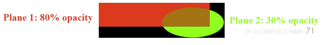
Many other planes can be added to either group. Color planes of the
same group are mixed together: Planes are stacked based on their order
and opacity. Opacity of 1st plane in a group does not affect color
mixing. There are 2 modes for mixing colors. See F7 key
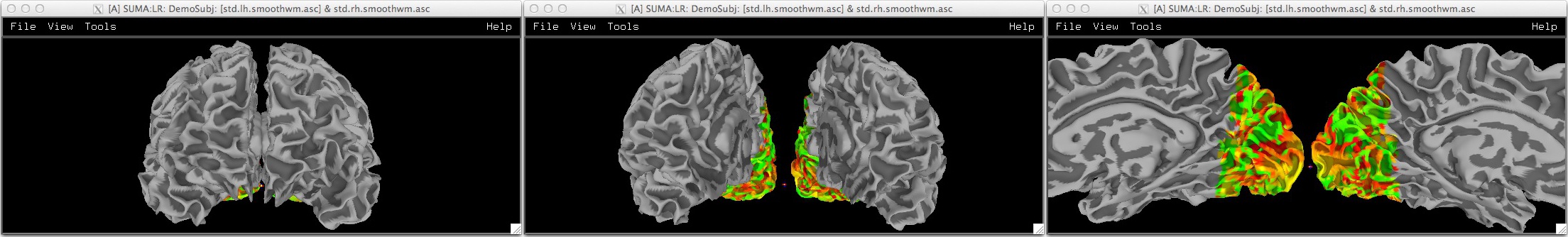
in SUMA.
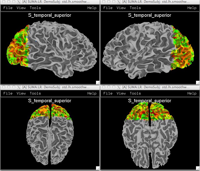
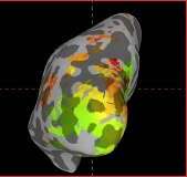
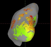
To demonstrate the layering of foreground and background planes, start
with a view of an inflated surface with some color overlay such as you
would get from talking to AFNI. Requires suma_demo:
Turn background plane(s) back on with b. Now you have
foreground atop background. You can still see the background
underneath the foreground – this is due to the background brightness
attenuation of the foreground colors.
Toggle background intensity attenuation off and on with a and see the effect on the resultant maps:
Prefixes fg: and bg: denote the plane’s group membership
Select lh.1D.col and lower its order with the Ord button
Select FuncAfni_0 and play with its opacity
Note: You can’t make a plane change its group membership, yet.
You can’t delete a loaded color plane yet, but you can reload it if it
changes on disk, or you can hide it with Dsp.
Turn 1 ON if you just want to see
the selected plane with no blending business from other planes. The
plane displayed would be the one whose label is shown in the surface
controller.
Test!
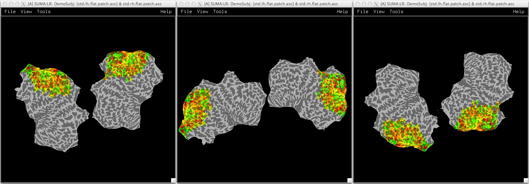
Find a way to flip between the mapping from AFNI and the mapping
(done with 3dVol2Surf
on the command line with script run_3dVol2Surf.)
Appreciate the differences between the two mappings.
Group: Usually the Subject’s ID. In the current SUMA
version, you can only have one group per spec file. All
surfaces read by SUMA must belong to a group.
NewSurface: A tag announcing the beginning of a set of
fields for a new surface.
SurfaceName or FreeSurferSurface: Name of the surface
file.
SurfaceFormat: ASCII or BINARY
SurfaceType: FreeSurfer, Caret, BrainVoyager, Ply, etc.
SurfaceState: Surfaces can be in different states such as
inflated, flattened, etc. The label of a state is arbitrary and
can be defined by the user. The set of available states must be
defined with StateDef at the beginning of
the Spec file.
StateDef: Used to define the various states. This must be
placed before any of the surfaces are specified.
Anatomical: Used to indicate whether surface is anatomically
correct (Y) or not (N). Anatomically correct surfaces are sent to
AFNI.
LocalDomainParent: Name of a surface whose mesh is shared by
other surfaces in the spec file.
The default for FreeSurfer surfaces is the smoothed gray
matter/ white matter boundary. For SureFit it is the fiducial
surface. Use SAME when the LocalDomainParent for a surface is
the surface itself.
EmbedDimension: Embedding Dimension of the surface, 2 for
surfaces in the flattened state, 3 for other.