9.6. Some 3dDeconvolve Notes¶

9.6.1. Overview ¶

These are notes by Bob Cox, from the great 3dDeconvolve Upgrades of 2004 and 2007. This page contains notes on various features added in that happy time.

Sections below will contain comments on underlying algorithms, option usage, and other words of wisdom that might be useful.

The current help page is for 3dDeconvolve is here.

The original 2004 notes page is here.

The original 2007 notes page is here.

9.6.2. `3dDeconvolve` Upgrades: Summer 2004 ¶

SVD for X-matrix pseudoinverse ¶

Gaussian elimination on the normal equations of X has been replaced by using the SVD to compute the X matrix pseudoinverse. This can be disabled using the -nosvd option. If the SVD solution is on, then all-zero -stim_file functions will NOT be removed from the analysis (unlike the -nosvd analysis).

The reason for not removing the all-zero regressors is so that GLTs and other scripts that require knowing where various results are in the output can still function.

One plausible case that can give all-zero regressors: a task with “correct” and “incorrect” results, you analyze these cases separately, but some subjects are so good they don’t have any incorrect responses.

The SVD solution will set the coefficient and statistics for an all-zero regressor to zero.

If two identical (nonzero) regressors are input, the program will complain but continue the analysis. In this case, each one would get half the coefficient, which only seems fair. However, your interpretation of such cases should be made with caution.

For those of you who aren’t mathematicians: the SVD solution basically creates the orthogonal principal components of the columns of the X matrix (the baseline and stimulus regressors), and then uses those to solve the linear system of equations in each voxel.

X-matrix condition numbers ¶

The X matrix condition number is now computed and printed. This can be disabled using the -nocond option. As a rough guide, if the matrix condition number is about 10^p, then round off errors will cause about p decimal places of accuracy to be lost in the calculation of the regression parameter estimates. In double precision, a condition number more than 10^7 would be worrying. In single precision, more than 1000 would be cause for concern. Note that if Gaussian elimination is used, then the effective condition number is squared (twice as bad in terms of lost decimal places); this is why the SVD solution was implemented.

The condition number is the ratio of the largest to the smallest singular value of X. If Gaussian elimination is used (-nosvd; see here), then this ratio is squared.

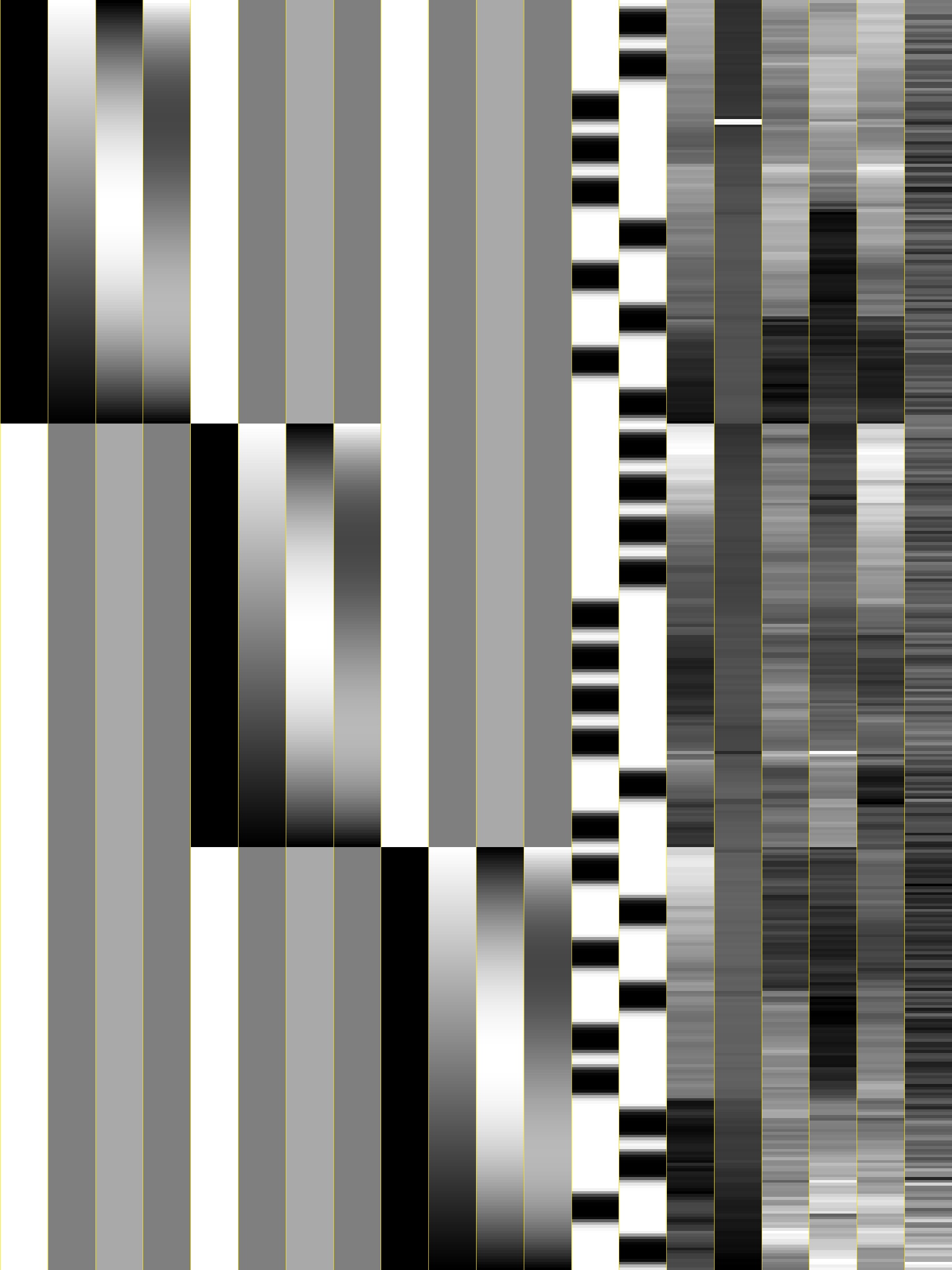
Option: `-xjpeg`¶

The new -xjpeg filename option will save a JPEG image of the columns of the regression matrix X into the given file.

X-matrix from Bootcamp example

Each column is scaled separately, from white=minimum to black=maximum.
Environment variable AFNI_XJPEG_COLOR determine the colors of the lines drawn between the columns.
- The color format is rgbi:rf/gf/bf, where each rf, gf and bf is a number between 0.0 and 1.0 (inclusive).
- For example, yellow would be rgbi:1.0/1.0/0.0.
- As a special case, if this value is the string none or NONE, then these lines will not be drawn.
- See here for getting color codes: https://rgbcolorpicker.com/0-1 (ignore the alpha value “a”).
Environment variable AFNI_XJPEG_IMXY determines the size of the image saved when via the -xjpeg option to 3dDeconvolve.
It should be in the format AxB:
- A is the number of pixels the image is to be wide (across the matrix rows)
- B is the number of pixels high (down the columns)
- For example:
```
setenv AFNI_XJPEG_IMXY 768x1024
```
Which means to set the x-size (horizontal) to 768 pixels and the y-size (vertical) to 1024 pixels. These values are the default, by the way.
If the first value A is negative and less than -1, its absolute value is the number of pixels across PER ROW.
If the second value B is negative, its absolute value is the number of pixels down PER ROW.
Usually there are many fewer columns than rows.

Warnings ¶

3dDeconvolve now checks for duplicate -stim_file names, and duplicate matrix columns. Only warning messages are printed – these are not fatal errors (at least, if the SVD solution is on).

Matrix Inputs ¶

Matrix inputs for the -glt option can now use a notation like 30@0 to indicate that 30 0s in a row are to be placed on the line. For example, if you have 10 runs catenated together, and you used -polort 2, then there are 30 baseline parameters to skip (usually) when specifying each GLT row.

The following is a sample matrix file with 34 entries per row:

30@0

1

-1

0

0

30@0

0

0

1

-1

Option: `-gltsym`¶

The new -gltsym gltname option lets you describe the rows of a GLT matrix using a symbolic notation.

Each stimulus is symbolized by its -stim_label option.
Each line in the gltname file corresponds to a row in the GLT matrix.

On each line should be a set of stimulus symbols, which can take the following forms (using the label Stim as the examplar):

Stim

put +1 in the matrix row for each lag of Stim

+Stim

put +1 in the matrix row for each lag of Stim (same as above)

-Stim

put -1 in the matrix row for each lag of Stim

Stim[2..7]

put +1 in the matrix for lags 2..7 of Stim

3*Stim[2..7]

put +3 in the matrix for lags 2..7 of Stim

Stim[[2..4]]

put +1 in the matrix for lags 2..4 of Stim in 3 successive rows of the matrix, as in:

1	0	0
0	1	0
0	0	1

... whereas Stim[2..4] would yield one matrix row

0

1

0

There can be no spaces or * characters in the stimulus symbols; each set of stimulus symbols on a row should be separated by one or more spaces. For example, the two multi-lag regressors entered with the options below.

-stim_label 1 Ear -stim_minlag 1 0 -stim_maxlag 1 5 \
-stim_label 2 Wax -stim_minlag 2 2 -stim_maxlag 2 7

This could have a GLT matrix row specified by:

+Ear[2..5] -Wax[4..7]

Which would translate into a matrix row like (zeros for the baseline):

0 0 1 1 1 1 0 0 -1 -1 -1 -1

Some comments:

With -gltsym, you do not have to specify the number of rows on the command line – the program will determine that from the file.
You can embed comment lines in the file – these are lines that start with the characters # or //.
If you want to access the polynomial baseline parameters for some bizarre reason, you can use the symbolic name Ort; otherwise, the GLT matrix elements corresponding to these parameters will all be set to 0, as in the example above.
A GLT can be expressed directly on the command line with an option of the form:
```
-gltsym 'SYM: +Ear[2..5] -Wax[4..7]'
```
where the SYM: that starts the string indicates that the rest of the string should be used to define the 1 row matrix. It is important that this string be enclosed in forward single quotes, as shown. If you want to have multiple rows specified, use the \ character to mark the end of each row, as in:
```
-gltsym 'SYM: +Ear[2..5] \ -Wax[4..7]'
```
You probably want to use the -glt_label option with -gltsym, as with -glt.
If you want to have the matrices generated by -gltsym printed to the screen, you can set environment variable AFNI_GLTSYM_PRINT to YES.

Legendre Polynomials ¶

Polynomial baseline functions now default to Legendre polynomials, which are more pleasantly behaved than the older power baseline functions. If you need the old power functions, you must use the -nolegendre option; this should only be the case if you use the baseline parameter estimates for some purpose.

For each block of contiguous data, the time range from first to last is scaled to the interval [-1,1]. The standard Legendre polynomials P_n(x) are then entered as baseline regressors, for n=0,1,...

Option: `-cbucket`¶

You can save ONLY the estimated parameters (AKA regression coefficients) for each voxel into a dataset with the new -cbucket cprefix option. This may be useful if you want to do some calculations with these estimates; you won’t have to extract them from the various statistics that are stored in the output of the -bucket bprefix option.

Option: `-xsave`¶

In combination with the old -bucket bprefix option, the new -xsave option saves the X matrix (and some other information) into file bprefix.xsave. Use this option when you first run 3dDeconvolve, if you think you might want to run some extra GLTs later, using the -xrestore option (below) – this is usually much faster than running the whole analysis over from scratch.

Option: `-xrestore`¶

The new -xrestore filename.xsave option will read the -xsave file and allow you to carry out extra GLTs after the first 3dDeconvolve run. When you use -xrestore, the only other options that have effect are -glt, -glt_label, -gltsym, -num_glt, -fout, -tout, -rout, -quiet, and -bucket. All other options on the command line will be ignored (silently). The original time series dataset (from -input) is named in the -xsave file, and must be present for -xrestore to work. If the parameter estimates were saved in the original -bucket or -cbucket dataset, they will also be read; otherwise, the estimates will be re-computed from the voxel time series as needed. The new output sub_bricks from the new -glt options will be stored as follows:

No -bucket option given in the -xrestore run will be stored at end of original -bucket dataset.
-bucket bbb option given in the -xrestore run will be stored in dataset with prefix “bbb”, which will be created if necessary; if “bbb” already exists, new sub-bricks will be appended to this dataset.

Option: `-input`¶

The -input option now allows input of multiple 3D+time datasets, as in:

-input fred+orig ethel+orig lucy+orig ricky+orig

Each command line argument after -input that does NOT start with a - character is taken to be a new dataset. These datasets will be catenated together in time (internally) to form one big dataset. Other notes:

You must still provide regressors that are the full length of the catenated imaging runs; the program will NOT catenate files for the -input1D, -stim_file, or -censor options.
If this capability is used, the -concat option will be ignored, and the program will use time breakpoints corresponding to the start of each dataset from the command line.

Progress Meter ¶

Unless you use the quiet option, 3dDeconvolve now prints a “progress meter” while it runs. When it is done, this will look as below where each digit is printed when 2% of the voxels are done.

++ voxel loop:0123456789.0123456789.0123456789.0123456789.0123456789.

Option: `-stim_times`¶

Direct input of stimulus timing, plus generation of a response model, with the new -stim_times option:

-stim_times k tname rtype

k and tname ¶

k is the stimulus index (from 1 to the -num_stimts value).

tname is the name of the file that contains the stimulus times (in units of seconds, as in the TR of the -input file). There are two formats for this file.

A single column of numbers, in which case each time is relative to the start of the first imaging run (“global times”).
If there are R runs catenated together (either directly on the command line, or as represented in the -concat option), the second format is to give the times within each run separately. In this format, the input file tname would have R rows, one per run; the times for each run take up one row. For example, with R=2:
```
12.3 19.8 23.7 29.2 39.8 52.7 66.6
21.8 32.7 41.9 55.5
```
These times will be converted to global times by the program, by adding the time offset for each imaging run.

N.B.: The times are relative to the start of the data time series as input to 3dDeconvolve. If the first few points of each imaging run have been cut off, then the actual stimulus times must be adjusted correspondingly (e.g., if 2 time points were excised with TR=2.5, then the actual stimulus times should be reduced by 5.0 before being input to 3dDeconvolve).
When using the multi-row input style, you may have the situation where the particular class of stimulus does not occur at all in a given imaging run. To encode this, the corresponding row of the timing file should consist of a single * character; for example, if there are 4 imaging runs but the kth stimulus only occurs in runs 2 and 4, then the tname file would look something like this:
```
*
3.2 7.9 18.2 21.3
*
8.3 17.5 22.2
```
In the situation where you are using multi-row input AND there is at most one actual stimulus per run, then you might think that the correct input would be something like:
```
*
*
30
*
```
However, this will be confused with the 1 column format, which means global times, and so this is wrong. Instead, you can put an extra * on one line with an actual stimulus, and then things will work OK:
```
*
*
30 *
*
```

rtype ¶

rtype specifies the type of response model that is to follow each stimulus. The following formats for rtype are recognized, along with the more modern types describe in the current version of the program help here.

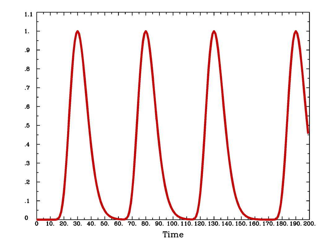
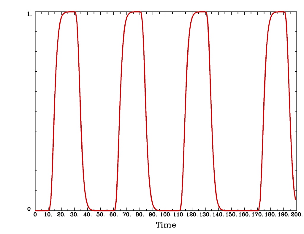
'GAM' is the response function $h_G(t;b,c) = (t/(bc))^b\,\exp(b-t/c)$ for the Cohen parameters $b=8.6, c=0.547$ . This function peaks at the value 1 at $t=bc$ , and is the same as the output of waver -GAM. See here for waver.

`GAM` output from `-xjeg`	`GAM` output from `1dplot`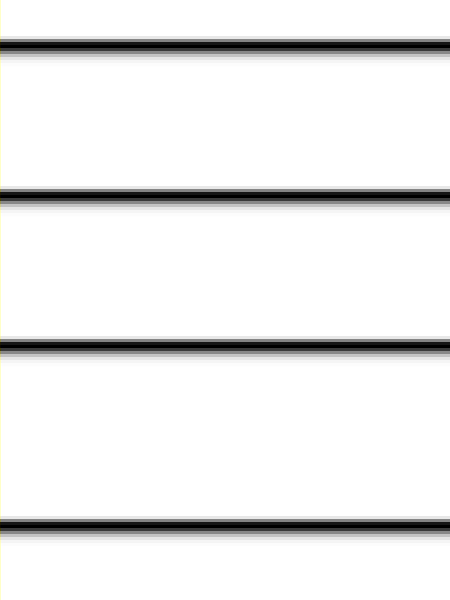

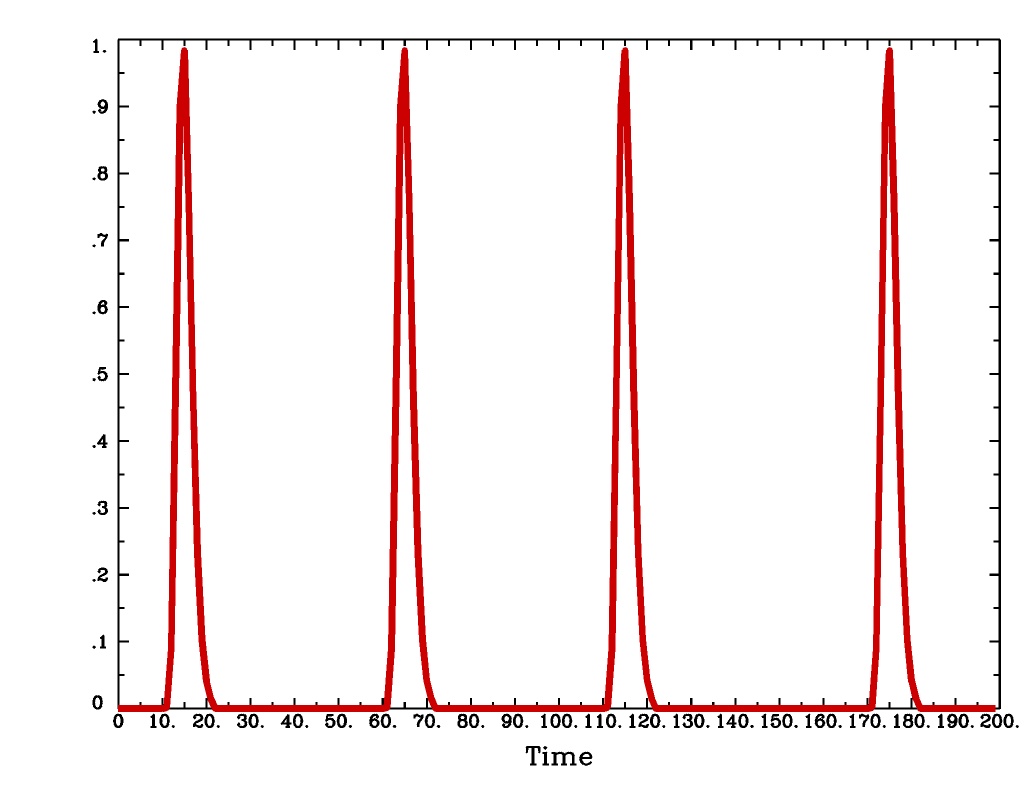
Plot generated with:

3dDeconvolve                                                  \
    -nodata 200 1.0 -num_stimts 1 -polort -1 -xjpeg gam_x.jpg \
    -local_times -x1D stdout:                                 \
    -stim_times 1 '1D: 10 60 110 170' 'GAM'                   \
  | 1dplot -THICK -one -stdin -xlabel Time  -jpg GAM_1d.jpg   \
        -DAFNI_1DPLOT_COLOR_01=red

'GAM(b,c)' is the same response function as above, but where you give the ‘b’ and ‘c’ values explicitly. The GAM response models have 1 regression parameter per voxel (the amplitude of the response).

`GAM(b,c)` output from `-xjeg`	`GAM(b,c)` output from `1dplot`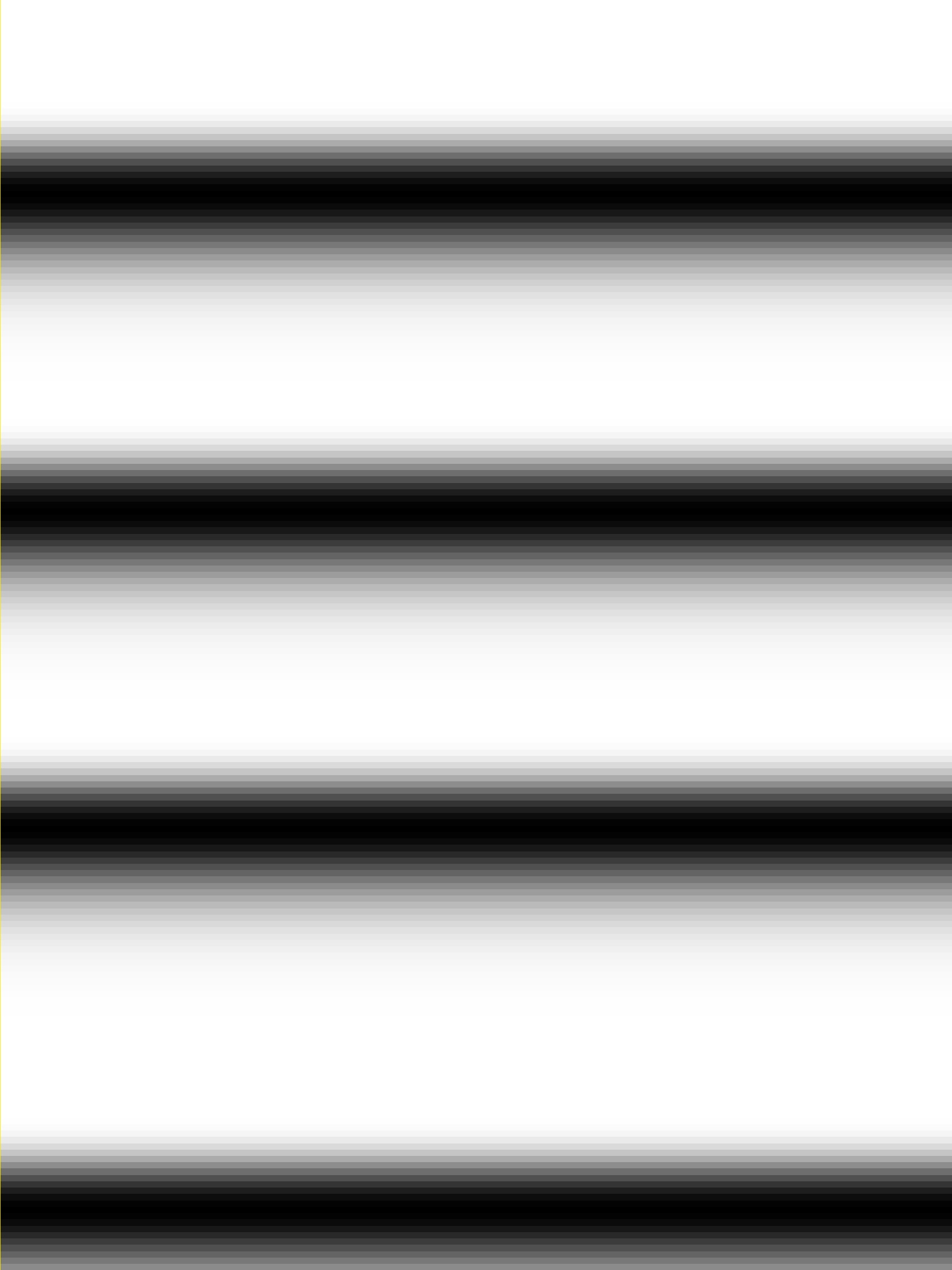

Plot generated with:

3dDeconvolve                                                     \
    -nodata 200 1.0 -num_stimts 1 -polort -1 -xjpeg GAMbc_x.jpg  \
    -local_times -x1D stdout:                                    \
    -stim_times 1 '1D: 10 60 110 170' 'GAM(10,2)'                \
  | 1dplot -THICK -one -stdin -xlabel Time -jpg GAMbc_1d.jpg     \
       -DAFNI_1DPLOT_COLOR_01=red

'SPMG2' is the SPM gamma variate regression model, which has 2 regression parameters per voxel. The basis functions are:

h_SPM,1(t) = exp(-t) [ t⁵/12 - t¹⁵/(6*15!) ]
h_SPM,2(t) = d/dt [ h_SPM,1(t) ]

`SPMG2` output from `-xjeg`	`SPMG2` output from `1dplot`

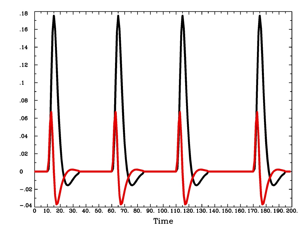
Plot generated with:

3dDeconvolve                                                    \
    -nodata 200 1.0 -num_stimts 1 -polort -1 -xjpeg SPMG2_x.jpg \
    -local_times -x1D stdout:                                   \
    -stim_times 1 '1D: 10 60 110 170' 'SPMG2'                   \
  | 1dplot -THICK -one -stdin -xlabel Time -jpg SPMG2_1d.jpg

'TENT(b,c,n)' is a tent function deconvolution model, ranging between times s+b and s+c after each stimulus time s, with n basis functions (and n regression parameters per voxel).
- A ‘tent’ function is just the colloquial term for a ‘linear B-spline’. That is tent(x) = max( 0 , 1-|x| )
- A ‘tent’ function model for the hemodynamic response function is the same as modeling the HRF as a continuous piecewise linear function. Here, the input ‘n’ is the number of straight-line pieces.
TENT(b,c,n) output from -xjeg

TENT(b,c,n) output from 1dplot

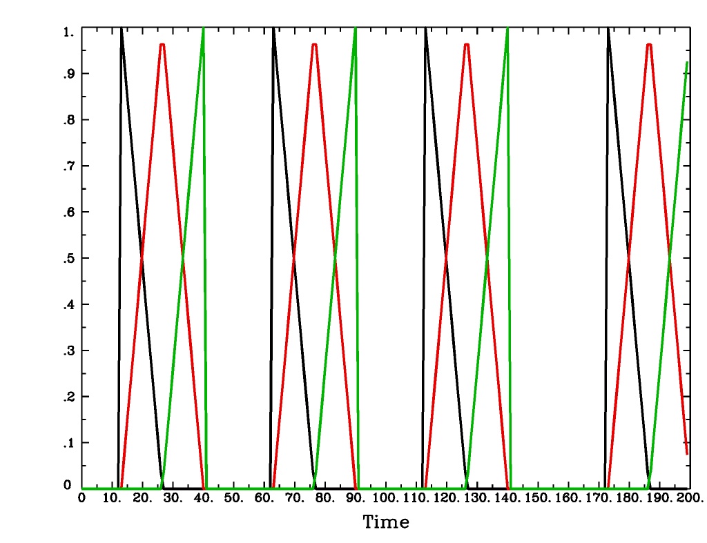
Plot generated with:
```
3dDeconvolve                                                    \
    -nodata 200 1.0 -num_stimts 1 -polort -1 -xjpeg TENT_x.jpg  \
    -local_times -x1D stdout:                                   \
    -stim_times 1 '1D: 10 60 110 170' 'TENT(3,30,3)'            \
  | 1dplot -thick -one -stdin -xlabel Time -jpg TENT_1d.jpg
```

'CSPLIN(b,c,n)' is a cubic spline deconvolution model; similar to the TENT model, but where smooth cubic splines replace the non-smooth tent functions.

`CSPLIN(b,c,n)` output from `-xjeg`	`CSPLIN(b,c,n)` output from `1dplot`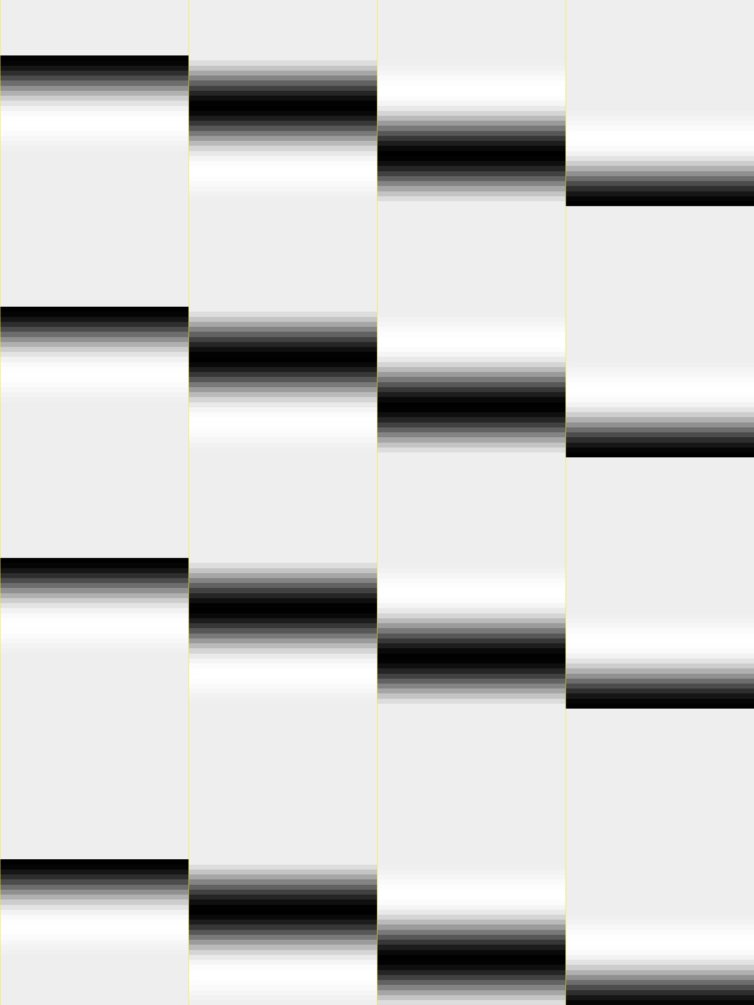

Plot generated with:

3dDeconvolve                                                     \
    -nodata 200 1.0 -num_stimts 1 -polort -1 -xjpeg CSPLIN_x.jpg \
    -local_times -x1D stdout:                                    \
    -stim_times 1 '1D: 10 60 110 170' 'CSPLIN(1,30,4)'           \
  | 1dplot -thick -one -stdin -xlabel Time -jpg CSPLIN_1d.jpg

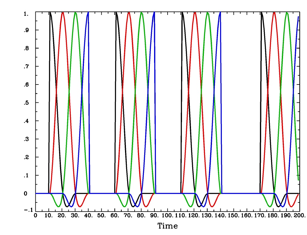
'SIN(b,c,n)' is a sin() function deconvolution model, ranging between times s+b and s+c after each stimulus time s, with n basis functions (and n regression parameters per voxel). The qth basis function, for q=1..n, is h_SIN,q(t) = sin(qπ(t-b)/(c-b)).

`SIN(b,c,n)` output from `-xjeg`	`SIN(b,c,n)` output from `1dplot`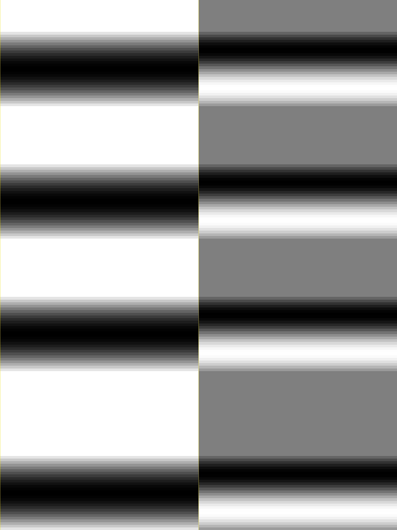

Plot generated with:

3dDeconvolve                                                  \
    -nodata 200 1.0 -num_stimts 1 -polort -1 -xjpeg SIN_x.jpg \
    -local_times -x1D stdout:                                 \
    -stim_times 1 '1D: 10 60 110 170' 'SIN(1,30,2)'           \
  | 1dplot -thick -one -stdin -xlabel Time -jpg SIN_1d.jpg

'POLY(b,c,n)' is a polynomial function deconvolution model, ranging between times s+b and s+c after each stimulus time s, with n basis functions (and n regression parameters per voxel). The qth basis function, for q=1..n, is h_POLY,q(t) = P_q(2(t-b)/(c-b)-1) where P_q(x) is the qth Legendre polynomial.

`POLY(b,c,n)` output from `-xjeg`	`POLY(b,c,n)` output from `1dplot`

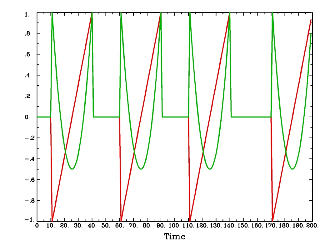
Plot generated with:

3dDeconvolve                                                   \
    -nodata 200 1.0 -num_stimts 1 -polort -1 -xjpeg POLY_x.jpg \
    -local_times -x1D stdout:                                  \
    -stim_times 1 '1D: 10 60 110 170' 'POLY(1,30,3)'           \
  | 1dplot -thick -one -stdin -xlabel Time -jpg POLY_1d.jpg

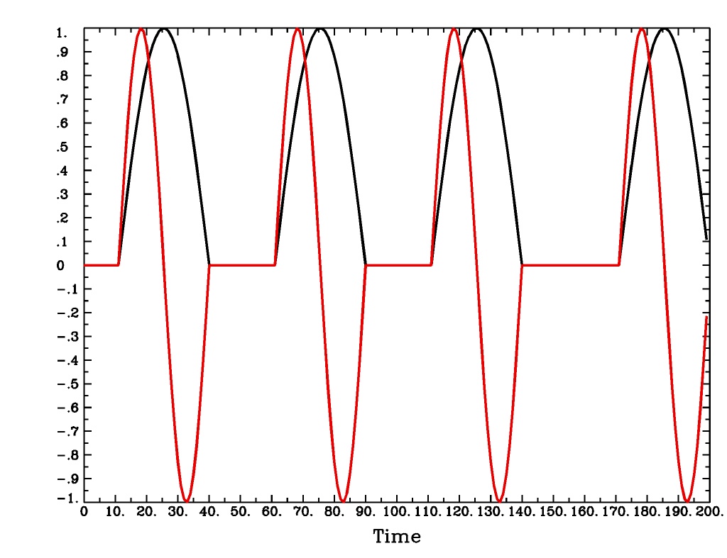
'BLOCK(d,p)' is a block stimulus of duration d starting at each stimulus time.
- The basis block response function is the convolution of a gamma variate response function with a ‘tophat’ function: $H(t) = \int_0^{min(t,d)} h(t-s) ds$ , where $h(t) = (t/4)^4\,\exp(4-t)$ ; $h(t)$ peaks at $t=4$ , with $h(4)=1$ , whereas $H(t)$ peaks at $t=d/(1-\exp(-d/4))$ . Note that the peak value of $H(t)$ depends on ‘d’; call this peak value $H_{peak}(d)$ .
- 'BLOCK(d)' means that the response function to a stimulus at time s is $H(t-s)$ for $t=s..s+d+15$ .
- 'BLOCK(d,p)' means that the response function to a stimulus at time s is $p\cdot H(t-s)/H_{peak}(d)$ for $t=s..s+d+15$ . That is, the response is rescaled so that the peak value of the entire block is ‘p’ rather than $H_{peak}(d)$ . For most purposes, the best value would be $p=1$ .
- 'BLOCK' is a 1 parameter model (the amplitude).
BLOCK(d,p) output from -xjeg

BLOCK(d,p) output from 1dplot

Plot generated with:
```
3dDeconvolve                                                    \
    -nodata 200 1.0 -num_stimts 1 -polort -1 -xjpeg BLOCK_x.jpg \
    -local_times -x1D stdout:                                   \
    -stim_times 1 '1D: 10 60 110 170' 'BLOCK(20,1)'             \
  | 1dplot -thick -one -stdin -xlabel Time -jpg BLOCK_1d.jpg  \
        -DAFNI_1DPLOT_COLOR_01=red
```

'EXPR(b,c) exp1 exp2 ...' is a set of user-defined basis functions, ranging between times s+b and s+c after each stimulus time s. The expressions are given using the syntax of 3dcalc, and can use the symbolic variables:
- 't' = time from stimulus
- 'x' = t scaled to range from 0 to 1 over the b..c interval
- 'z' = t scaled to range from -1 to 1 over the b..c interval
- An example, which is equivalent to 'SIN(0,35,3)', is 'EXPR(0,35) sin(PI*x) sin(2*PI*x) sin(3*PI*x)'. Expressions are separated by blanks, and must not contain whitespace themselves. An expression must use at least one of the symbols ‘t’, ‘x’, or ‘z’, unless the entire expression is the single character “1”.

The basis functions defined above are not normalized in any particular way. The -basis_normall option can be used to specify that each basis function be scaled so that its peak absolute value is a constant. For example -basis_normall 1 will scale each function to have amplitude 1. Note that this scaling is actually done on a very fine grid over the entire domain of t values for the function, and so the exact peak value may not be reached on any given point in the actual FMRI time series.

Note that it is the basis function that is normalized, not the convolution of the basis function with the stimulus timing!
The -basis_normall option must be given before any -stim_times options to which you want it applied!

If you use a -iresp option to output the hemodynamic (impulse) response function corresponding to a -stim_times option, this function will be sampled at the rate given by the new -TR_times dt option. The default value is the TR of the input dataset, but you may wish to plot it at a higher time resolution. (The same remarks apply to the -sresp option.)

Since the parameters in most models do not correspond directly to amplitudes of the response, care must be taken when using GLTs with these.

The parameters for GAM, TENT, CSPLIN, and BLOCK do corresond directly to FMRI signal change amplitudes.
I NEED TO THINK THIS THROUGH SOME MORE (Says Bob)

Next to be implemented (someday): an option to compute areas under the curve from the basis-function derived HRFs.

More changes are on the way - RWCox - 22 Sep 2004 - Bilbo and Frodo Baggins’ birthday!

The -nodata option now works with the -stim_times option.

However, since -stim_times needs to know the number of time points (NT) and the time spacing (TR), you have to supply these values after the -nodata option if you are using -stim_times.
For example: -nodata 114 2.5 to indicate 114 points in time with a spacing of 2.5 s.

9.6.3. `3dDeconvolve` Updates: 2007 ¶

Small changes: to the defaults, new options, etc.¶

-nobout and -full_first are now the defaults. These changes mean that if you want the $\beta$ weights for the baseline parameters in the output -bucket dataset, you have to specify -bout on the command line. If you want the full-model statistics to appear last in the dataset, you have to specify -nofull_first on the command line.
Even if you do not give the -fout option on the command line (indicating you do not want F-statistics for various hypotheses to be calculated), the program will still compute the full model F-statistics. If you don’t want that for some reason, you have to use the new -nofullf_atall option.
If you do not give a -bucket option on the command line, then the program will act as if you had given -bucket Decon. (This is known as the “Ah need a bucket” change, with apologies to KFC.)
The program now always outputs (to a file) the regression matrix X, even if you don’t give a -x1D option. The default filename will be the same as the -bucket prefix, with the suffix .x1D added.
- The matrix file format has been slightly altered to store column labels in XML-style comments in the header. (Previously, the matrix was just written out as an array of unlabeled numbers.) These labels will be useful in an upcoming regression matrix analysis program being planned by Ziad Saad. They are also useful in the new program 3dSynthesize (cf. infra).
3dDeconvolve used to fail with the -nodata option combined with -stim_times. This crash should be a thing of the past.
- When using -nodata, the program needs to know the length of the (non-existent) imaging data (number of TRs) and it also needs to know the TR. The simplest and best way to specify these values is to put them immediately after the -nodata option; for example -nodata 300 2.5 to indicate 300 time points with TR=2.5 s.
- If you don’t do the above, then if you use -nlast, that value (+1) will be used as the number of TRs. If you don’t give the TR in some way, then the default -nodata TR is 1.0 s. This TR is unimportant if you only use -stim_file, but is crucial if you use -stim_times with -nodata or with -input1D.
New option -float (or -datum float) can be used to make all the output datasets be stored in floating point format. In the past, only scaled shorts were possible, and the limited (16-bit) precision of these sometimes caused problems. Shorts are still the default, but at some point in the future I may change the default to floats – if/when this happens, the option -short can be used if you like the more compact format.
The program now reports when -stim_times time values are out of the time span of the dataset. These are not fatal errors, but can help notify you to potential problems of your timing files. (This problem is known as the PSFB syndrome – it’s not as bad as the Mike Beauchamp syndrome, but try to avoid it.)
The labels for the -bucket output dataset sub-bricks have been changed slightly to be more consistent and readable (e.g., Tstat instead of t-st to indicate a t-statistic).
3dDeconvolve now computes a recommended -polort value (1 degree for every 150 s of continuous imaging). If your input value is less than this, a non-fatal WARNING message is printed. If you use -polort A, then the program will automatically choose the polynomial degree to use for detrending (AKA high pass filtering).
A new CSPLIN() model for -stim_times is now available. This function is a drop-in replacement for TENT(), with the same 3 arguments. The basis functions are cardinal cubic splines, rather than cardinal linear splines. CSPLIN() will produce smoother looking HRF curves, if plotted with -TR_times less than the dataset TR. (As always, if you are going to change your analysis methodology, run some data the old way and the new way, then compare the results to make sure you understand what is happening!)

Detection and processing of matrix errors; new `-GOFORIT` option ¶

3dDeconvolve now makes several more checks for “bad things” in the regression matrix.
- Besides checking the full matrix condition number, it also checks several sub-matrices: the signal sub-model, the baseline sub-model, the -polort sub-model, and the -stim_base sub-model.
- Each check is printed out and labeled as to how good the program “thinks” it is. Potentially bad values are flagged with ** BEWARE **
- N.B.: 3dDeconvolve’s condition number is not exactly the same as that computed by Matlab. 3dDeconvolve first scales the matrix columns to have L²-norm = 1, and then computes the condition number from the ratio of the extreme singular values of that matrix. This method prevents the pathology of saying that the matrix diag(1,10^–6) is ill-conditioned.
- Other “bad things” that the program checks for include duplicate stimulus filenames, duplicate regression matrix columns, and all zero matrix columns.

If “bad things” are detected in the matrix (each will be flagged in the text printout with a warning message containing the symbols ‘!!’), then 3dDeconvolve will not carry out the regression analysis. However, if you give the command line option -GOFORIT, then the program will proceed with the analysis. I strongly recommend that you understand the reason for the problem(s), and don’t just blindly use -GOFORIT all the time.

To help disentangle the ERROR and WARNING messages (if any) from the rest of the text output, they are now also output to a file named 3dDeconvolve.err.

New option for censoring time points ¶

The -CENSORTR option lets you specify on the command line time points to be removed from the analysis. It is followed by a list of strings; each string is of one of the following forms:

`37`	remove global time index #37
`2:37`	remove time index #37 in run #2
`37..47`	remove global time indexes #37-47
`37-47`	same as above
`2:37..47`	remove time indexes #37-47 in run #2
`'*:0-2'`	remove time indexes #0-2 in all runs

Time indexes within each run start at 0.
Run indexes start at 1 (just be to confusing, and also to be compatible with afni_proc.py).
Multiple -CENSORTR options may be used, or multiple -CENSORTR strings can be given at once, separated by spaces or commas.
N.B.: Under the above rules, 2:37,47 means index #37 in run #2 and then global time index #47; it does not mean index #37 in run #2 and then index #47 in run #2. To help catch this possible misuse, the program will print a warning message if you use some -CENSORTR strings with run numbers and some without run numbers.

New program `3dSynthesize` for creating 3D+time datasets ¶

This program combines the $\beta$ weights stored in the -cbucket output from 3dDeconvolve, and the regression matrix time series stored in the -x1D output, to produce model fit time series datasets. 3dDeconvolve itself has the -fitts option to produce the full model fit in each voxel. 3dSynthesize can be used to produce model fits from subsets of the full model.

In the examples below, suppose that fred+orig is the output from -cbucket and that fred.x1D is the output from -x1D. Also suppose that there were two stimulus classes, given labels Face and House in 3dDeconvolve using -stim_label options.

Baseline sub-model:
```
3dSynthesize                                        \
    -cbucket fred+orig -matrix fred.x1D             \
    -select baseline -prefix fred_baseline
```
For example, you could subtract fred+baseline+orig from the FMRI data time series, using 3dcalc, to get a signal+noise dataset with no baseline. This combination of programs would be one way to detrend a multi-run dataset in a logically consistent fashion.

Baseline plus Face stimulus sub-model (but not the House stimulus):

3dSynthesize                                        \
    -cbucket fred+orig -matrix fred.x1D             \
    -select baseline Face prefix fred_Face

Baseline plus House stimulus sub-model (but not the Face stimulus):

3dSynthesize                                        \
    -cbucket fred+orig -matrix fred.x1D             \
    -select baseline House prefix fred_House

In general, if you want to “Double Plot” the resulting dataset on top of the original time series dataset (with the Dataset #N plugin), you’ll need the baseline model component so that the 3dSynthesize output is on the same magnitude scale for graphing.
For further details, see the -help output from 3dSynthesize: available here.

[25 Jun 2007] Censoring

3dDeconvolve and 3dSynthesize have been modified to work when the 3dDeconvolve run using a time point censoring option (i.e., -censor and/or -CENSORTR). The matrix files output by 3dDeconvolve (which files are now renamed to end in .xmat.1D) have information about which time points were censored. 3dSynthesize can use that information to generate sub-bricks to fill in those time points which are missing in the actual matrix. The options are:

`-cenfill zero`	rfill censored time points with zeros [the new default]
`-cenfill nbhr`	fill censored time points with the average of their non-censored time neighbors
`-cenfill none`	rdon’t put sub-bricks in for censored time points [what the program used to do]

Another option is to use the new -x1D_uncensored filename option in 3dDeconvolve to output an uncensored version of the regression matrix, then use that matrix as the input the 3dSynthesize. Then the model fit that you choose will be computed at all the time points.

9.6.4. Amplitude Modulated FMRI regression analysis ¶

Analysis of event-related FMRI data when the amplitude of each event’s BOLD response might depend on some externally observed data.

Conceptual Introduction ¶

When carrying out an FMRI experiment, the stimuli/tasks are grouped into classes. Within each class, the FMRI-measurable brain activity is presumed to be the same for each repetition of the task. This crude approximation is necessary since FMRI datasets are themselves crude, with low temporal resolution and a low contrast-to-noise ratio (i.e., the BOLD signal change is not very big). Therefore multiple measurements of the “same” response are needed to build up decent statistics.

In many experiments, with each individual stimulus/task a separate measurement of subject behavior is taken; for example, reaction time, galvanic skin response, emotional valence, pain level perception, et cetera. It is sometimes desirable to incorporate this Amplitude Modulation (AM) information into the FMRI data analysis.

Binary AM ¶

If the AM were binary in nature (“on” and “off”), one method of carrying out the analysis would be to split the tasks into two classes, and analyze these stimulus classes separately (i.e., with two -stim_times options). The statistical test for activation ignoring the AM would then be a 2 DOF F-test, which could be carried out in 3dDeconvolve by using a 2 row GLT. The contrast between the two conditions (“on−off”) could be carried out with a 1 row GLT. For example:

3dDeconvolve ...                                                    \
    -stim_times 1 regressor_on.1D  'BLOCK(1,1)' -stim_label 1 'On'  \
    -stim_times 2 regressor_off.1D 'BLOCK(1,1)' -stim_label 2 'Off' \
    -gltsym 'SYM: On \ Off' -glt_label 1 'On+Off'                   \
    -gltsym 'SYM: On -Off'  -glt_label 2 'On-Off' ...

(A realistic 3dDeconvolve command line would, of course, have more options to specify the input and output filenames, etc.) The above example assumes that each case (“on” and “off”) is being analyzed with simple (fixed-shape) regression – short 1-second blocks of activity.

Nothing more will be said here about binary AM, since it is just a standard application of 3dDeconvolve; the only (small) difference is that the stimulus class to which each individual stimulus is assigned is determined during the FMRI data acquisition itself, rather than determined by the investigator before the imaging session.

Continuous AM ¶

More complex is the case where the AM measurement values fall onto a continuous (or finely graded discrete) scale. One form of analysis is then to construct two regressors: the first being the standard constant-amplitude-for-all-events-in-the-same-class time series, and the second having the amplitude for each event modulated by that event’s AM value (or some function of the AM value). To make these two regressors be orthogonal, it is best to make the modulation be proportional to the difference between each event’s AM value and the mean AM value for that stimulus class.

The new -stim_times_AM2 option is designed to make this type of analysis easy. The ‘AM’ in the option suffix indicates that amplitude modulation for each time is expected in the input timing file. The ‘2’ indicates that 2 regressors will be generated from 1 stimulus timing file.

The stimulus timing file for -stim_times_AM2 has a slightly different format than the stimulus timing file for the standard -stim_times option. Each stimulus time in the _AM2 file must have an amplitude “married” to it. For example:

10*5 30*3 50*2 70*7 90*-3

This indicates that the stimuli at times 10, 30, 50, 70, and 90 have amplitudes of 5, 3, 2, 7, and -3 (respectively). Note that if a stimulus time is given without an amplitude, the amplitude will be taken to be zero and 3dDeconvolve will print a warning message. (N.B.: the ‘*’ separator can also be the ‘x’ character, if that is more convenient.)

The program 1dMarry can be used to “glue” two .1D formatted files together to produce a file appropriate for -stim_times_AM2. With the -divorce option, it can also split up a “married” file into 2 separate files – one with the times and one with the amplitudes. These features makes it relatively straightforward to run a standard 3dDeconvolve analysis with -stim_times and also the new -stim_times_AM2 type of analysis.

The same response models available with the standard -stim_times option are also usable with -stim_times_AM2. Two regression matrix columns will be generated for _AM2 for each one column specified by the response model (e.g., 'BLOCK(1,1)' generates 1 column normally, and 2 columns when used with _AM2). The first column will be created by giving equal weight (1) to each event in the stimulus timing file. The second column will have each event weighted by the difference between its individual amplitude and the mean of all amplitudes in the timing file. The significance of the output $\beta$ weight for this second column (e.g., given by using the -tout option) can be used to map regions that are (linearly) sensitive to the amplitude information. The significance of the combined $\beta$ weights for the two columns (e.g., given by using the -fout option) can be used to map regions that are sensitive the stimulus class as a whole.

It can be useful and enlightening to plot the columns of the regression matrix that correspond to the equal-weight and variable-weight model time series generated by -stim_times_AM2. For this purpose, program 1dplot can be applied to subsets of the .x1D file output by 3dDeconvolve.

It is possible to use the option -stim_times_AM1 if you want to just generate a single regression model where each event is simply scaled by its associated amplitude. There will be no separation of the model into the constant and varying components. I do not recommend this, for reasons given below, but the option is available. (If you can think of a good reason to use this option for analysis of FMRI time series, please let me know!)

Deconvolution with Amplitude Modulation ¶

It is also legal to use a deconvolution model (e.g., 'TENT()') with -stim_times_AM2. However, you must realize that the program will compute a separate HRF shape for the AM component of the response from the mean component. It is not possible to specify that the AM component has the same shape as the mean component, and just has a different response amplitude – that would be a nonlinear regression problem, and 3dDeconvolve isn’t that flexible. Also, at present, the -iresp option will not output the HRF for the AM component of a -stim_times_AM2 deconvolution model. Nor have I actually tried using AM deconvolution myself on real data. If you are going to try to do this, you should (a) understand what you are doing, and (b) consult with someone here.

Why Use 2 Regressors?¶

One user asked the following question: “Can’t I just use the AM weighted-regressor in the model by itself? Why do you have to include the standard (mean amplitude) regressor in the full model to investigate the effect of event amplitude values?” In other words, why not use -stim_times_AM1?

The reasoning behind separating the regressor columns into 2 classes (mean activation and AM-varying activation) is

to allow for voxels where the amplitude doesn’t affect the result, and

to allow for a cleaner interpretation; in voxels where both regressors have significant weight, you can use the coefficient ( $\beta$ weight) of the first regressor as the mean activation level, and the coefficient of the second as the dependence of the activation level on the amplitude.

A numerical example might help elucidate:

Suppose that you have 6 events, to be simple, and that the amplitudes for these events are {1, 2, 1, 2, 1, 2}, with mean=1.5. Now suppose you have a voxel that IS active with the task, but whose activity is not dependent on the amplitude at all. Say its activation level with each task is 6, so the “activity vector” (i.e., the BOLD response amplitude for each event) is {6, 6, 6, 6, 6, 6}. This vector is highly correlated with the AM vector {1, 2, 1, 2, 1, 2} (cc=0.9486), so you will get a positive activation result at this voxel when using a single regressor. You can’t tell from the regression if this voxel is sensitive to the amplitude modulation or not.

But if you use 2 regressors, they would be proportional to {1, 1, 1, 1, 1, 1} and {-0.5, +0.5, -0.5, +0.5, -0.5, +0.5} (the differences of each event amplitude from the mean of 1.5). The first regression vector is perfectly correlated with the “activity vector” {6, 6, 6, 6, 6, 6} and the second regression vector is not correlated with the activity at all. So you would get an activation result saying “this voxel was activated by the task, but doesn’t care about the amplitude”. You cannot make such a dissection without using 2 regressors.

Even if you don’t care at all about such non-AM-dependent voxels, you must still include them if you think this may be a significant effect in the data. You have to model the data as it presents itself. In a sense, the constant-activation model is like the baseline model (e.g., -polort stuff), in that it must be included in the fit since it does occur, but you are free to ignore it as you will. Interpreting the results is your problem.

What about Losing Degrees of Freedom?¶

If you are concerned about losing degrees of freedom, since you will be adding regressors but not data, then I would run the analysis twice. Once with the mean regressors only, and then one with the mean and the variable regressors. Then decide if the maps from the mean regressors in the two cases differ markedly. My guess is that they will not, if you have a decent number of events in each case (30+). If they do not differ too much, then you are safe to use the double regressor (AM2) analysis. If they do differ a lot (e.g., you lose a lot of mean regressor activation when you set the F-statistic p-values the same), then you probably can’t use the double regressor analysis. But it is easy enough to try.

You can open two AFNI controllers, and view the single and double regressor analyses side-by-side. You can set the threshold sliders to be locked together in p-value (using Edit Environment on variable AFNI_THRESH_LOCK). This should help you decide very quickly if the two results look the same or not – same, that is, from the viewpoint of interpreting the results. The maps will of course not be identical, since they will have been calculated with different models.

Caveats and Issues ¶

One problem with the above idea is that one may not wish to assume that the FMRI signal is any particular function of the event amplitude values. I don’t know at this time how to deal with this issue in the context of linear regression. For example, the “linear in event amplitude” model could be extended to allow for a quadratic term (-stim_times_AM3?), but it is highly unclear that this would be useful. Some sort of combination of regression analysis with a mutual information measurement might be needed (to quantify if the BOLD response is “predictable” from the AM information), but I don’t fully know how to formulate this idea mathematically.

9.6. Some 3dDeconvolve Notes¶

9.6.1. Overview ¶

9.6.2. `3dDeconvolve` Upgrades: Summer 2004 ¶

SVD for X-matrix pseudoinverse ¶

X-matrix condition numbers ¶

Option: `-xjpeg`¶

Warnings ¶

Matrix Inputs ¶

Option: `-gltsym`¶

Legendre Polynomials ¶

Option: `-cbucket`¶

Option: `-xsave`¶

Option: `-xrestore`¶

Option: `-input`¶

Progress Meter ¶

Option: `-stim_times`¶

k and tname ¶

rtype ¶

9.6.3. `3dDeconvolve` Updates: 2007 ¶

Small changes: to the defaults, new options, etc.¶

Detection and processing of matrix errors; new `-GOFORIT` option ¶

New option for censoring time points ¶

New program `3dSynthesize` for creating 3D+time datasets ¶

9.6.4. Amplitude Modulated FMRI regression analysis ¶

Conceptual Introduction ¶

Binary AM ¶

Continuous AM ¶

Deconvolution with Amplitude Modulation ¶

Why Use 2 Regressors?¶

What about Losing Degrees of Freedom?¶

Caveats and Issues ¶

Table of Contents

This Page

Quick search