Structural Equation Modeling (SEM) or Path Analysis
Document Actions
Introduction
Path Analysis is a causal modeling approach to exploring the correlations within a defined network. The method is also known as Structural Equation Modeling (SEM), Covariance Structural Equation Modeling (CSEM), Analysis of Covariance Structures, or Covariance Structure Analysis. In FMRI data analysis it has been applied to visual system, language production, motor attention, memory system, etc.. Historically it is an approach more often used as confirmatory (hypothesis testing) than exploratory (descriptive or model searching), more model-driven than data-driven, and more "causal" than correlative.
The hypothetical model in path analysis usually involves two kinds of variables: observable/manifest (endogenous or dependent) variable and latent (exogenous or non-observable) variables. Observable variables serve as indicators of the underlying construct represented by the observable variables, and latent variables are usually theoretical constructs that cannot be observed directly. In FMRI the observable variables are BOLD time series at those regions of interest, while it usually does not involve any latent variables.
There are two goals of path analysis: (1) understanding patterns of correlations among the regions; (2) explaining as much of the regional variation as possible with the model specified. Different from statistical testing in other techniques, such as multiple regression and ANOVA, the focus in path analysis is usually on a decision about the whole model: reject, modify, or accept it?
A few noteworthy points regarding path analysis:
* Interpretation of path coefficients: First of all, they are not
correlation coefficients. Suppose we have a network with a path
connecting from region A to region B. The meaning of the path
coefficient theta (e.g., 0.81) is this: if region A increases by one
standard deviation from its mean, region B would be expected to
increase by 0.81 its own standard deviations from its own mean while
holding all other relevant regional connections constant. With a path
coefficient of -0.16, when region A increases by one standard deviation
from its mean, region B would be expected to decrease by 0.16 its own
standard deviations from its own mean while holding all other relevant
regional connections constant.
* Requirement for large sample size? < 100: small; 100-200: medium.
* An alternative model might account for the proposed model equally well if not better.
* Keep in mind there is a difference between a statistical model of reality and reality itself (Kline, 2005).
* Statistical causal modeling (including SEM) does not prove causation.
* Specification error of omitting ROIs from a path analysis is that estimates of causal effects of ROIs included in the model may be inaccurate if some ROIs are omitted that co-vary with those in the model, and the error could be either underestimation (more likely) or overestimation.
* One assumption of path analysis, measurement error for exogenous variables, is hardly true in FMRI.
* Uncertain about the directionality of an effect? (1) Try alternative models with different directonalities: (2) Include reciprocal effects. The first is preferred. However, it is possible some models equally fit the data, thus no statistical basis for model selection among alternatives. Inclusion of reciprocal effect makes the analysis non-recursive (thus more difficult to analyze). (3) Include all possible paths? Limit on degrees of freedom, which has to be positive so that the model would be identifiable.
1dSEM in the most recent AFNI package is specifically written for path analysis in the context of FMRI field based on Bullmore et al. [1] and Stein and Meyer-Lindenberg [2]. A big difference here from the conventional path analysis is that the residual error variances are estimated prior to the analysis instead of being treated as unknown parameters. The main reason is that the sample size is relatively small in FMRI data.
For more discussion, see G. Chen, et al., Vector autoregression, structural equation modeling, and their synthesis in neuroimaging data analysis, Comput. Biol. Med. (2011), doi:10.1016/j.compbiomed.2011.09.004
A script for preprocessing and running SEM
To make life easier, we created a tcsh script
(updated Dec 11, 2008) that contains all the steps described below except ROI time
series extraction. First make sure you have the most recent version of
AFNI on your computer. If you have n subjects and m ROIs, you need one input file for each of those n subjects, in which you store the m ROI time series as m columns, plus a file specifying the connections. To run the script, do something like this:
tcsh -x SEMscript.csh subj1.1D subj2.1D ... subj15.1D thetas.1D
Again the last file in the command line, thetas.1D, stores a matrix of mxm (m
= number of ROIs) whose specifications were discussed above. Also, at
the end of the script, there are 3 command lines for running SEM in 3
different modes: model validation, tree model, and forest search. So
you may want to make some modifications there.
Details of running SEM
The following is a suggested scheme for obtaining input data for 1dSEM. It is assumed that all subjects have gone through exactly the same experiment design, and the time series have been extracted at those regions of interest for each subject from the input file for individual subject analysis (motion corrected and scaled properly). If some subjects don't share the same time series, you can stack all subjects' data, and then calculate the covariance or correlation matrix, but then you may have to modify the following steps to adopt the new situation.
You may consider using 3dSynthesize (and 3dcalc) to remove effects of no interests such as baseline, head motion, task effects of no interest, physiological fluctuations, etc..
Suppose there are 15 subjects, 5 ROI's with 300 TR's in each time series, totaling 15 X 5 = 75 times series: ts#_Subj*.1D
(1) Compute eigentimeseries for each ROI.
For each ROI, run singular value decomposition (SVD) on an n X T matrix (time series of all subjects) using 1dsvd (n = number of subjects, T = number of TR's in the extracted time series):
1dsvd ts#_Subj1.1D ts#_Subj2.1D .. ts#_Subjn.1D (# is the region serial number)
The output on the screen looks like this (15 subjects and 300 TR's):
++ 1dsvd input vectors:
00..00: ts_Subj1.1D
01..01: ts_Subj2.1D
...
14..14: ts_Subjn.1D
++ Data vectors [A]:
--------- --------- ---------
00: 0.15000 0.00000 ... 0.00000
01: 0.27300 0.16000 ... 0.53000
...
299: 0.01000 0.22500 ... 0.00000
++ Left Vectors [U]:
25.639 7.9888 ... 0.5319
------------ ------------ ------------
00: -0.38698 0.075116 ... -0.090827
01: -0.09261 0.033281 ... -0.077916
...
299: -0.42006 -0.040904 ... 0.35085
++ Right Vectors [V]:
25.63904 7.98879 ... 0.53188
--------- --------- --------------
00: -0.52292 0.64472 ... 0.55758
01: -0.65014 0.12138 ... -0.75006
...
14: -0.55126 -0.75472 ... 0.35568
++ Pseudo-inverse:
--------- --------- --------- ----
00: 0.01331 0.00150 ... 0.02793
01: 0.02114 0.01112 ... -0.02553
...
14: -0.01018 -0.00799 ... 0.03334
The SVD decomposition is in the format of A = USV', where S is a diagonal matrix consisting of singular values s1, s2, ..., s15 of A (or the square roots of the eigenvalues of A'A.) These singular values are shown above for both left and right matrices in the output in descending order.
Extract the first column from left matrix U which corrresponds to the largest singular value s1, and save it as sv_nn.1D (nn represents the ROI index). This vector is also the corresponding eigenvector of A'A. Plot out sv_nn.1D (1dplot), and verify whether it has a pattern more or less matching up the frequency of the experiment design.
(2) For each ROI re-sign left singular vectors sv*.1D
Obtain average time course of the ROI:
3dMean -prefix ts_mean_nn Subj*_ts_nn.1D
set dotp = `3ddot -dodot sv_nn.1D ts_mean_nn.1D`
1deval -a sv_nn.1D -expr "step(-$dotp)*(-a)+step($dotp)*a" >svc_nn.1D
The last command corrects the sign of sv.1D if the output (a single number, the dot product) from 3ddot is negative.
(3) Calculate covariance or correlation matrix
Correlation matrix is usually used because of arbitrary scaling issue in the BOLD signal.
Once steps 2 and 3 are done for all ROI's, estimate the inter-regional covariance matrix based on singular vector identified above
1ddot -dem -cov -terse svc_1.1D svc_2.1D ... svc_5.1D (5 ROIs in this example)
Alternatively, you can get the covariance coefficient matrix by running
1ddot -dem -cov -terse ts_mean_1.1D ts_mean_2.1D ... ts_mean_5.1D
If you prefer to use the correlation matrix, do the following
1ddot -dem -terse svc_1.1D svc_2.1D ... svc_5.1D
or
1ddot -dem -terse ts_mean_1.1D ts_mean_2.1D ... ts_mean_5.1D
(4) Calculate residual error variances for each ROI
psi = Σsi2-s12 (basically the sum of those singular values squared without the first - principal - one)
where s1, s2, ..., s15 are singular values of A in step 1.
Or if you obtained correlation matrix during the previous step, use
psi = 1 - s12/Σsi2
(5) Obtain effective degrees of freedom
Use 3ddot to get the first order autocorrelation coefficient ar_i for i-th ROI
3ddot -demean svc#.1D'{0..298}' svc#.1D'{1..299}' (# is the serial region number)
or,
3ddot -demean ts#_mean.1D'{0..298}' ts1_mean.1D'{1..299}' (# is the serial region number)
The effective degrees of freedom is estimated as
(T/P) Σ(1-ar_i)/(1+ar_i) (you can use a calculator such as ccalc)
where T = number of time points in each time series, P = number of ROI's
(6) Use results from steps 3, 4, and 5 as input for 1dSEM.
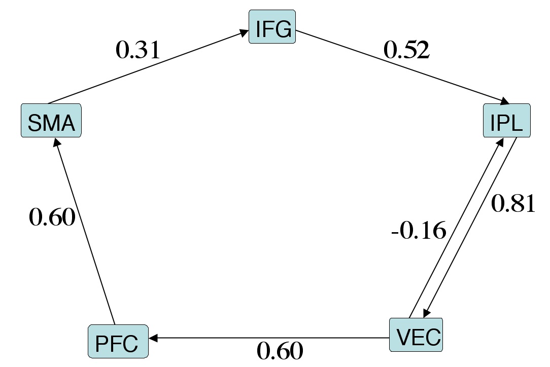
There are two basic modes of analysis in 1dSEM: model validation and model search. With model validation, you can test whether a theoretical network can stand against the path analysis. Suppose we have a model of 5 regions in the brain like this (focus on the path connections and ignore those path coefficients for the moment)
First create a text file testthetas.1D specifying the connections
# VEC PFC SMA IFG IPL
VEC 0 0 0 0 1
PFC 1 0 0 0 0
SMA 0 1 0 0 0
IFG 0 0 1 0 0
IPL 1 0 0 1 0
Save the correlation matrix from step 4 as file testcorr.1D
1 0 0 0 0
0.661 1 0 0 0
0.525 0.66 1 0 0
0.486 0.507 0.437 1 0
0.731 0.63 0.558 0.517 1
and the residual error variances from step 5 as file testpsi.1D
0.825
0.868
0.87
0.881
0.851
Then run 1dSEM (number 30 at the end of the script is from step 6)
1dSEM -theta testthetas.1D -C testcorr.1D -psi testpsi.1D -DF 30 -limits -1 1
with the following output on the screen
++ Program 1dSEM: AFNI version=AFNI_2007_01_15_xxxx [32-bit]
++ Authored by: Daniel Glen, Gang Chen
Finding optimal theta values
++ Total number of iterations 82429
++ Cost is 0.429081
++ Chi Square = 12.4434
Connection coefficients matrix: 5 x 5
01: 0.0000 0.0000 0.0000 0.0000 0.8076
02: 0.5974 0.0000 0.0000 0.0000 0.0000
03: 0.0000 0.5961 0.0000 0.0000 0.0000
04: 0.0000 0.0000 0.3144 0.0000 0.0000
05: -0.1589 0.0000 0.0000 0.5231 0.0000
The estimated path coefficients are shown in the above figure.
On the other hand if we want to adopt the model search mode looking for a 'best model' that fits the data, replace file testthetas.1D with the following matrix (check 1dSEM -help for definitions)
# VEC PFC SMA IFG IPL
VEC 0 2 2 2 2
PFC 2 0 2 2 2
SMA 2 2 0 2 2
IFG 2 2 2 0 2
IPL 2 2 2 2 0
and run the following
1dSEM -model_search -theta testthetas_ms.1D -C testcorr.1D -psi testpsi.1D -nrand 10 -DF 30 -stop_cost 0.1 -grow_all -max_paths 3 -limits -1 1
Output is something like
++ Program 1dSEM: AFNI version=AFNI_2006_06_30_1332 [32-bit]
++ Authored by: Daniel Glen, Gang Chen
nmodels to try is 20
theta_init_mat matrix: 5 x 5
# VEC PFC SMA IFG IPL
VEC 0.0000 2.0000 2.0000 2.0000 2.0000
PFC 2.0000 0.0000 2.0000 2.0000 2.0000
SMA 2.0000 2.0000 0.0000 2.0000 2.0000
IFG 2.0000 2.0000 2.0000 0.0000 2.0000
IPL 2.0000 2.0000 2.0000 2.0000 0.0000
Finding optimal theta values
Total number of iterations 147957
max i,j = 0, 4 with cost = 1.87853, ntheta = 1
Connection coefficients matrix: 5 x 5
# VEC PFC SMA IFG IPL
VEC 0.0000 0.0000 0.0000 0.0000 0.7310
PFC 0.0000 0.0000 0.0000 0.0000 0.0000
SMA 0.0000 0.0000 0.0000 0.0000 0.0000
IFG 0.0000 0.0000 0.0000 0.0000 0.0000
IPL 0.0000 0.0000 0.0000 0.0000 0.0000
Finding optimal theta values
Total number of iterations 247056
max i,j = 1, 2 with cost = 1.37668, ntheta = 2
Connection coefficients matrix: 5 x 5
# VEC PFC SMA IFG IPL
VEC 0.0000 0.0000 0.0000 0.0000 0.7310
PFC 0.0000 0.0000 0.6600 0.0000 0.0000
SMA 0.0000 0.0000 0.0000 0.0000 0.0000
IFG 0.0000 0.0000 0.0000 0.0000 0.0000
IPL 0.0000 0.0000 0.0000 0.0000 0.0000
Finding optimal theta values
Total number of iterations 310515
max i,j = 4, 2 with cost = 1.0108, ntheta = 3
Connection coefficients matrix: 5 x 5
# VEC PFC SMA IFG IPL
VEC 0.0000 0.0000 0.0000 0.0000 0.7310
PFC 0.0000 0.0000 0.6600 0.0000 0.0000
SMA 0.0000 0.0000 0.0000 0.0000 0.0000
IFG 0.0000 0.0000 0.0000 0.0000 0.0000
IPL 0.0000 0.0000 0.5580 0.0000 0.0000
Finding optimal theta values
Total number of iterations 370922
max i,j = 3, 4 with cost = 0.707411, ntheta = 4
Connection coefficients matrix: 5 x 5
# VEC PFC SMA IFG IPL
VEC 0.0000 0.0000 0.0000 0.0000 0.7310
PFC 0.0000 0.0000 0.6600 0.0000 0.0000
SMA 0.0000 0.0000 0.0000 0.0000 0.0000
IFG 0.0000 0.0000 0.0000 0.0000 0.5170
IPL 0.0000 0.0000 0.5580 0.0000 0.0000
Finding optimal theta values
Total number of iterations 438186
max i,j = 1, 0 with cost = 0.5501, ntheta = 5
Connection coefficients matrix: 5 x 5
# VEC PFC SMA IFG IPL
VEC 0.0000 0.0000 0.0000 0.0000 0.7310
PFC 0.4342 0.0000 0.4321 0.0000 0.0000
SMA 0.0000 0.0000 0.0000 0.0000 0.0000
IFG 0.0000 0.0000 0.0000 0.0000 0.5170
IPL 0.0000 0.0000 0.5580 0.0000 0.0000
Finding optimal theta values
Total number of iterations 750521
max i,j = 2, 3 with cost = 0.491374, ntheta = 6
Connection coefficients matrix: 5 x 5
# VEC PFC SMA IFG IPL
VEC 0.0000 0.0000 0.0000 0.0000 0.7310
PFC 0.4342 0.0000 0.4321 0.0000 0.0000
SMA 0.0000 0.0000 0.0000 0.2667 0.0000
IFG 0.0000 0.0000 0.0000 0.0000 0.4028
IPL 0.0000 0.0000 0.4618 0.0000 0.0000
*** Theoretically speaking the range of the path coefficients can be anything, but most of the time they do fall into [-1, 1]. To save runtime, the default values for -limits are set with -1 and 1, but if the result hits the boundary, increase them under option -limits and re-run the analysis.
*** To make life easier, we created a tcsh script (July 10, 2007) that contains all the above steps except ROI time series extraction. First make sure you have the most recent version of AFNI on your computer. If you have n subjects and m ROIs, you need one input file for each of those n subjects, in which you store the m ROI time series as m columns, plus a file specifying the connections. To run the script, do something like this:
tcsh -x SEMscript.csh subj1.1D subj2.1D ... subj15.1D thetas.1D
Again the last file in the command line, thetas.1D, stores a matrix of mxm (m = number of ROIs) whose specifications were discussed above. Also, at the end of the script, there are 3 command lines for running SEM in 3 different modes: model validation, tree model, and forest search. So you may want to make some modifications there.
Other packages
1. sem package in R, a free software environment for statistical computing and graphics [Download basic package - either the appropriate binary for your platform or the source code; Set up path; Install sem by implementing the following at R prompt: install.packages("sem",dependencies=TRUE); Try: library(sem) If it doesn't complain, everything is in the right order.] (manual)
2. A Matlab package by Douglas Steele (Matlab required)
3. Mplus has a free demo version with limitation of up to 6 dependent variables, 2 independent variables and 2 between variables in two-level analysis - Microsoft Windows
4. LISREL by Scientific Software International Inc. (student version free) - Microsoft Windows
5. AMOS (Analysis of Moment Structures) by SPSS, Inc. (Free student version limited to 8 observed variables and 54 parameters) - Microsoft Windows
6. CALIS (Covariance Analysis and Linear Structural ) procedure of SAS/STAT 8 - Microsoft Windows
7. EQS - Microsoft Windows
8. Mx Graph (FREE) - Microsoft Windows
Acknowlegement
We sincerely thank Andreas Meyer-Lindenberg and Jason Stein for their generous help during the development of this program.
References
[1] Bullmore, E. T., Horwitz, B., Honey, G. D., Brammer, M. J., Williams, S. C. R., Sharma, T., How Good is Good Enough in Path Analysis of fMRI Data? NeuroImage 11, 289-301 (2000).
[2] Stein, J.L., Wiedholz, L.M., Bassett, D.S., Weinberger, D.R., Zink, C.F., Mattay, V.S., Meyer-Lindenberg, A. (2007). “A Validated Network of Effective Amygdala Connectivity” NeuroImage 36: 736–745.
[3] SEM wiki
[4] http://www2.chass.ncsu.edu/garson/pa765/structur.htm


