12.14.2. Manifold ways to make+view spheres in SUMA
Description
This tutorial starts with:
a list of coordinates representing the center of spheres
a dset that provides a background/grid (here, MNI space)
and shows how to:
make+view spheres various ways in SUMA.
Survey of approaches
Spherical objects can be rendered in 4 general ways in suma (plus
some extra variants, noted in the script/examples).
NIDO: NeuroImaging Displayable Objects
There’s a demo for this in the distribution (@DO_examples), and I created a fun script for April Fool’s day that shows one sphere. These objects aren’t clickable in suma; they are only for display. The @DO_examples script needs a little modification for recent Mac OS to keep the screen controller open first. The April Fool’s Day posting here was for fun, but it does have a serious use - like yours.
Manufactured spherical surfaces (2 main kinds)
These are all clickable. That means clicking on a sphere identifies the node in some way. The coordinate can also be shared with the afni GUI if the two programs are talking to each other. Here again, you can do this multiple ways:
CreateIcosahedron - create an icosahedron or project to a sphere. The RAVE software (R Analysis and Visualization of intracranial EEG Data) by the Beauchamp lab uses this approach:
From volumetric datasets of spheres or real electrode geometry, as seen in CT images of ECOG. The ALICE software creates “spheres” based on the CT images or positions marked. The spheres are all made in the volume at the resolution of the dataset, so the conversion to a surface by IsoSurface is a little rough. These can be indexed sequentially as a “merged” surface of multiple surfaces, and colored by color maps or color planes in suma. For the ALICE software, all the electrodes, usually about 100, are colored separately. As each is selected, we turn off or dim the color by manipulating the color map where the sphere index is loaded (1-100) and then colored initially with a niml dataset, then colored with a color map suitable for ROI indices. The color planes offer an alternative way to color a surface; each node index can be colored separately.
ALICE: A tool for automatic localization of intra-cranial electrodes for clinical and high-density grids Mariana P. Branco, et al., 2017. Journal of Neuroscience Methods 301 DOI: 10.1016/j.jneumeth.2017.10.022.
Direct volumetric display
This is the least sophisticated way, but it is also the easiest. Make spheres in a volume with
3dUndump, each with a separate value for the sphere. There will be 4 columns in the input to 3dUndump for the xyz coordinates and the value to assign to the sphere. Show in suma withsuma -vol myspheres+orig. Render withsumaor even withafni’s Render plugin.Graph nodes object
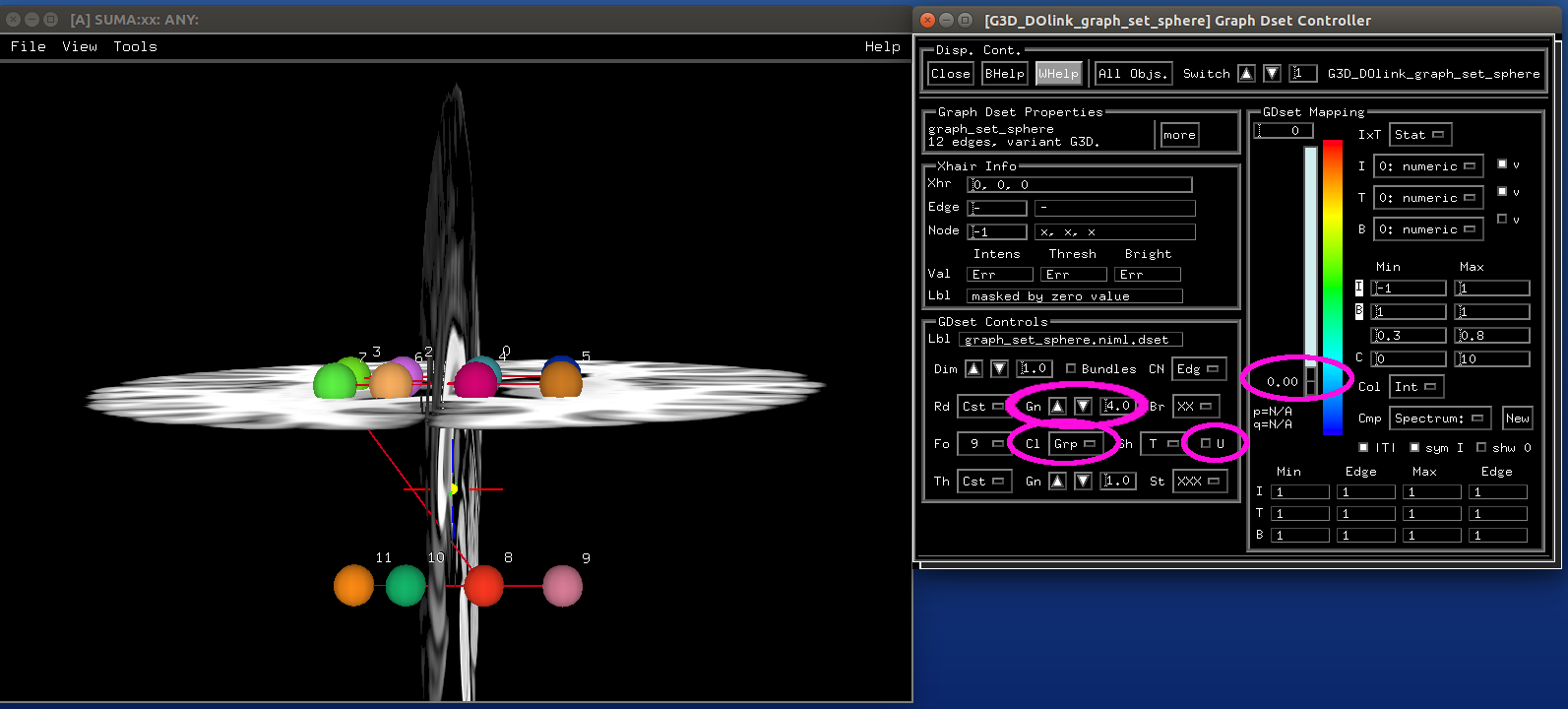
SUMA can also display “graphs”: essentially, nodes connected by edges. The nodes themselves are spheres, and thus they also count as a method for displaying those geometrical forms. The “bonus” aspect of this approach is that the edges can provide additional information/relationships among the spherical ROIs, such as structural or functional properties (connections, correlation, FA value, etc.). This has been useful in displaying atlas connections, for example in the D99 macaque atlas work (Reveley et al., 2017).
“Three-dimensional digital template atlas of the macaque brain” Reveley, Gruslys, Ye, Samaha, Glen, Russ, Saad, Seth, Leopold, Saleem, 2017. Cerebral Cortex, 27(9):4463-4477, https://doi.org/10.1093/cercor/bhw248”
Example Setup
You can download the individual script and supplementary files for running this demo here:
The pieces of this demo are also shown one-by-one below, so one can read along with them.
Files provided here include:
- sphere_coords.1D
a list of (x, y, z) coordinates that represent the centers of some spheres.
- ROI_i256.1D.cmap
a “colormap”, here a list of (R, G, B) color specifications. This one was made by hitting the “w” over the ROI_i256 colorbar in the SUMA object controller.
- demo_suma_spheres.tcsh
a script file to run all the commands, making spheres and displaying
sumacommands to view them (can be copy+pasted into terminal). Various warnings abound when running this script, but those are ignorable. The script can be run with:tcsh demo_suma_spheres.tcsh
Running the examples
Setup
This first step is just to create some additional files that we will need (the set of ROIs) and want (a skull-stripped anatomical) for the demo.
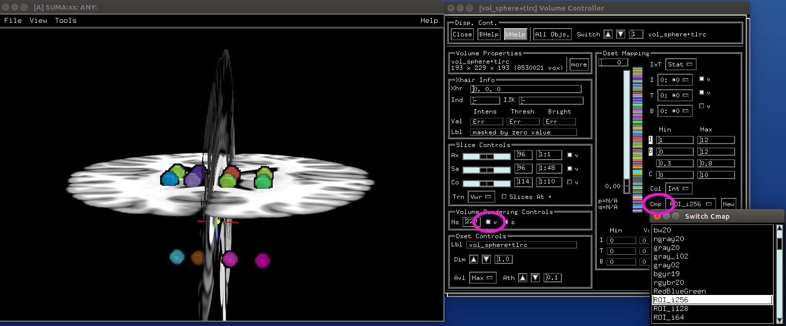
- show code y/n -Make volumes and display directly in SUMA
- show code y/n -sphere_00_vol.png |
|---|
|
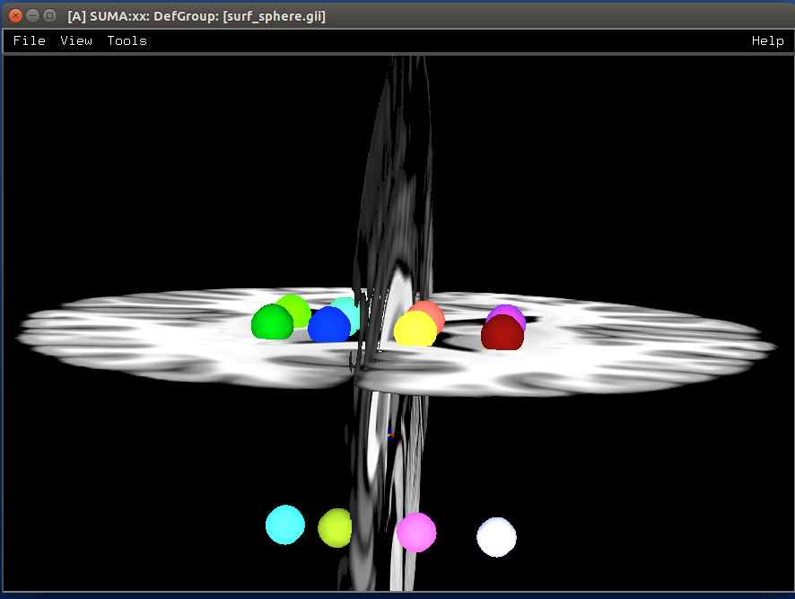
Make isosurfaces of the volumetric ROIs
- show code y/n -sphere_01_surf.png |
|---|
|
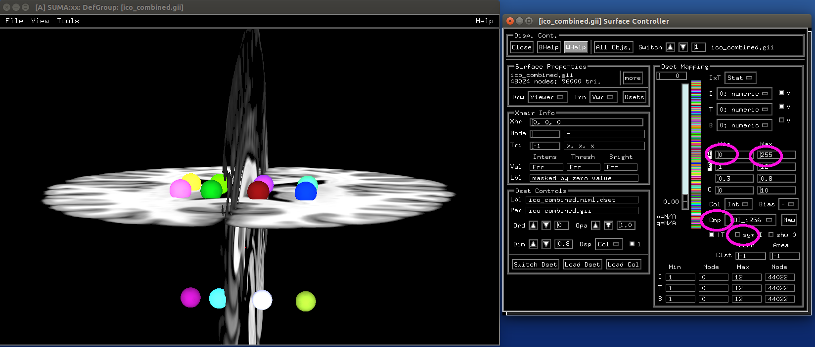
Make icosahedrons
- show code y/n -sphere_02_ico.png |
|---|
|
Make NIML Displayable Objects (Nidos)
- show code y/n -sphere_03_nido.png |
|---|
|
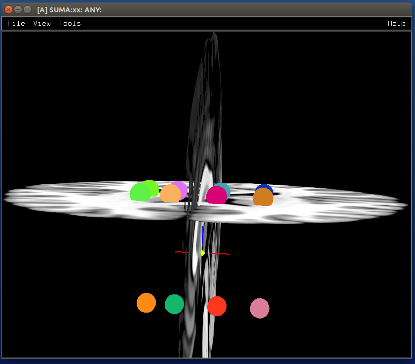
Spheres from graph views
- show code y/n -sphere_04_graph.png |
|---|
|