12.5.8. Post-preproc, II: mapping ROIs to DTI space
Overview
We might be interested in bringing other data into the processed
DWI/DT space. For example, we could have FreeSurfer (FS) surfaces and
parcellations from an anatomical T1w volume (and we do!), which have
already been brought into AFNI+SUMAable formats by
@SUMA_Make_Spec_FS. We can choose to bring just the volumetric
part of that (e.g., the segmentation+parcellation NIFTI files), or we
could bring both the volumes and surfaces. For the latter, this can
include the “*.gii” surfaces themselves, as well as the supplementary
information in the “*.niml.dset” files (such as the
annotation/labelling of nodes) and the “*.spec” files (which describe
how all the surface states relate and which annotation files go with
each).
The above describes the role of fat_proc_map_to_dti. In the
parlance of our times, we create a transformation map to the DWI’s
[0]th volume from the FS-output T1w volume, and then we can
apply that mapping to the other “follower” volume, surface,
supplementary, etc. files. The transformation is a 12 DOF linear
affine transform (made using 3dAllineate).
One specifies the followers by their category. For volume files, one can select whether the dset contains integers that should stay integers (possibly with labeltables) with nearest neighbor (“NN”) resampling, or whether it has floating points values that can be interpolated (with “wsinc5”). For surfaces, one specifies surface files, supplementary NIML dsets and specification files separately; however, we note that it only makes sense to map, say, *.spec files if one has matching surfaces and *.niml.dset files...
Note
In this example we map from a FS-processed T1w volume to DT space, bringing along FS parcellation maps and surfaces as followers.
However, one could also use this program to bring, say, FMRI data into DT space, since most FMRI processing pipelines involve aligning EPI to the subject’s anatomical. One could make a map from the subject’s T1w anatomical and have the FMRI maps be follower dsets.
fat_proc_map_to_dti
Proc: One specifies a source (here, the skull-stripped “brain.nii”
anatomical from FreeSurfer) and a base (the reference  file
that is likely the [0]th brick in the post-TORTOISE DWI data set) for
making the transformation.
file
that is likely the [0]th brick in the post-TORTOISE DWI data set) for
making the transformation.
One then can specify volumetric and surfacey follower data sets by
category. Here, we select all the “renumbered” parcellation
volumetric files (see @SUMA_renumber_FS, which is run as part of
@SUMA_Make_Spec_FS for more info); many of these aren’t likely to
be directly useful since they contain maps of “unknown” or “other”
regions from FS, but they don’t take up much disk space when
compressed. These will all have auto-snapshot images made of them in
the new space.
Finally, we chose to map the higher resolution standardized mesh
surfaces (“ld 141”) from @SUMA_Make_Spec_FS, as well as their
accompanying *.niml.dsets and *.spec files, for simpler viewing
later. At present, there is not auto-snapshot capability for SUMA
viewing; we describe some simplish ways to use the *.spec files to
view the output, below.
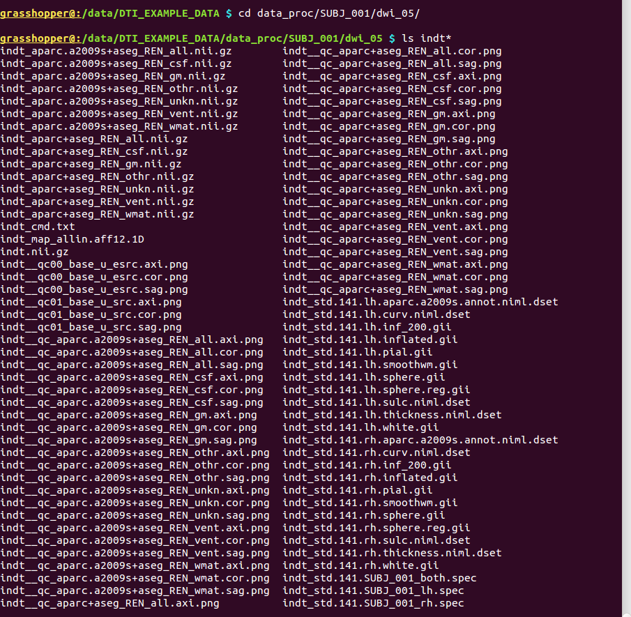
This was all done by running (note the use of wildcards in selecting many dsets per follower type):
# I/O path, same as above, following earlier steps
set path_P_ss = data_proc/SUBJ_001

fat_proc_map_to_dti                                                \
    -source          $path_P_ss/anat_02/SUMA/brain.nii             \
    -followers_NN    $path_P_ss/anat_02/SUMA/aparc*_REN_*.nii.gz   \
    -followers_surf  $path_P_ss/anat_02/SUMA/std.141.*.gii         \
    -followers_ndset $path_P_ss/anat_02/SUMA/std.141.*.niml.dset   \
    -followers_spec  $path_P_ss/anat_02/SUMA/std.141.*.spec        \
    -base            $path_P_ss/dwi_05/dwi_dwi.nii.gz'[0]'         \
    -prefix          $path_P_ss/dwi_05/indt
-> putting all of the outputs into the existing ‘data_proc/SUBJ_001/dwi_05/’ directory, since all the files there should be in the same DT space:
Directory substructure for example data set |
|---|
|
Output from fat_proc_map_to_dti. |
Outputs of |
|
|---|---|
indt_cmd.txt |
textfile, copy of the command that was run, and location |
indt.nii.gz |
volumetric NIFTI file, 3D; the “source” dset (here, the skull-stripped T1w output from FS) in the DT space; how well this aligns to the “base” diffusion volume determines the appropriateness of the transformation/mapping. |
indt_map_allin.aff12.1D |
textfile, the 12 DOF linear affine registration parameters for the mapping process; gets applied to all the volumetric followers, and its inverse gets applied to the surface followers (AFNI and SUMA transforms work in opposite ways). |
indt_aparc+aseg_REN_*.nii.gz |
volumetric NIFTI files, 3D; each contains a parcellation and/or
segmentation map from the FS “2000” parcellation, renumbered by
|
indt_aparc.a2009s+aseg_REN_*.nii.gz |
volumetric NIFTI files, 3D; each contains a parcellation and/or
segmentation map from the FS “2009” parcellation, renumbered by
|
indt_std.141.*.gii |
surface GIFTI files; FS surfaces translated over, in this case
the “ld 141” version of the standardized surface from
|
indt_std.141.*.niml.dset |
NIML format surface data sets; these contain things like
parc/seg labeltables, etc. (made by |
indt_std.141.*.spec |
specification files for defining relative states of surface
dsets, as well as matching the *.niml.dset label dsets with
the appropriate surfaces (made by |
indt__qc00_base_u_esrc.*.png |
autoimages, multiple slices within single volume; ulay = reference [0]th DWI volume (b/w); olay = FS structural file brain.nii, edgified (red); use these images to judge the quality of alignment. |
indt__qc01_base_u_src.*.png |
autoimages, multiple slices within single volume; ulay = reference [0]th DWI volume (b/w); olay = FS structural file brain.nii (translucent, “plasma” colorbar); use these images to judge the quality of alignment. |
indt__qc_aparc+aseg_REN_*.*.png, indt__qc_aparc.a2009s+aseg_REN_*.*.png |
autoimages, multiple slices within single volume; ulay = reference [0]th DWI volume; olay = FS parcellation/segmentation maps for a given tissue grouping/classification (translucent, “ROI_i256” colorbar); can also use these images to judge the quality of alignment, as well as the parcellation/segmentation itself. |
Autoimages of |
(just axi and sag views) |
|---|---|
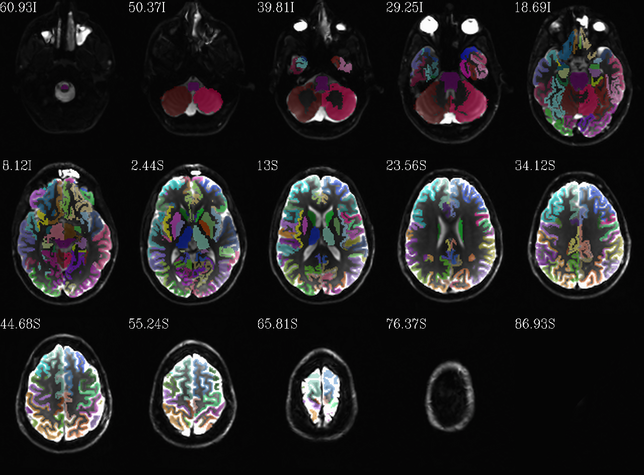
|

|
FS “2000” parc/seg map: the GM ROIs from AFNI renumbering (translucent olay) [0]th DWI volume as (b/w ulay). |

|

|
FS “2009” parc/seg map: the GM ROIs from AFNI renumbering (translucent olay) [0]th DWI volume as (b/w ulay). |

|

|
FS “2009” parc/seg map: the WM ROIs from AFNI renumbering (translucent olay) [0]th DWI volume as (b/w ulay). |

|

|
FS “2009” parc/seg map: the CSF ROIs from AFNI renumbering (translucent olay) [0]th DWI volume as (b/w ulay). |

|

|
FS “2009” parc/seg map: the ventricle ROIs from AFNI renumbering (translucent olay) [0]th DWI volume as (b/w ulay). |
Tracking + surface viewing: AFNI+SUMA example
Here is an example of using the data from the fat_proc_dwi_to_dt
(from HERE) and fat_proc_map_to_dti
(from HERE) functions for
visualization in AFNI+SUMA together. More in-depth descriptions of
tracking capabilities with 3dTrackID are given HERE, including a description of mini-probabilistic tracking in
relation to other modes. More in-depth descriptions of SUMA
visualization are generally demonstrated HERE, with
some specific reference to FATCAT demo examples HERE.
Both AFNI and SUMA can receive “key-press”-type information from the command line, so that you can adjust the viewers and change things that you would normally click or key-press in the GUI from scripts. This functionality is known as “driving”. Some description of driving SUMA are provided HERE, with lists of drivable functionalities HERE. Lists of AFNI drivable functions are given HERE. You can also check out more FATCAT-specific examples in the FATCAT Demo, which is obtainable as described HERE.
Note
We give a brief example here of using some basic SUMA capability in viewing surfaces+tract information, with additional AFNI-volume info. Ziad Saad, as the main author of SUMA, deserves a huge amount of thanks for these capabilities.
Proc A: we will do a basic mini-probabilistic tracking through the whole brain. First, we erode the whole brain mask obtained by automasking the T2w anatomical, because it contains parts of the skull still, and we prefer to avoid the little erroneous stuff that would appear there. So, the following could be run in the directory containing all the DT parameters (here ‘data_proc/SUBJ_001/dwi_05/’):
# erode (= dilate negatively) the WB mask to avoid skull stuff
3dmask_tool                                  \
    -dilate_inputs -2                        \
    -inputs dwi_mask.nii.gz                  \
    -prefix dwi_mask_ERODE2.nii.gz

# basic whole-brain, mini-prob tracking in it.
3dTrackID                                    \
    -mode MINIP                              \
    -mini_num 5                              \
    -mask dwi_mask_ERODE2.nii.gz             \
    -netrois dwi_mask_ERODE2.nii.gz          \
    -dti_in dt                               \
    -prefix TTT                              \
    -uncert dt_UNC.nii.gz                    \
    -logic OR                                \
    -alg_Nseed_X 1                           \
    -alg_Nseed_Y 1                           \
    -alg_Nseed_Z 1                           \
    -no_indipair_out
-> producing the following files:
Directory substructure for example data set |
|---|

|
Files output from WB mask erosion with 3dmask_tool and mini-probabilistic tracking with 3dTrackID. |
Proc B: Then, we set a couple environment variables and load up AFNI and SUMA to view the results. We include volumetric, surface and tract data sets. We use the fun capability of AFNI and SUMA to “talk” to each other in order to send information back and forth in the viewers: the outlines of the surfaces from SUMA appear in the AFNI windows, and some overlay coloration from AFNI will appear on the surfaces in SUMA:
# port for AFNI-SUMA communications, and end all other chatter on it
set cport = 12
@Quiet_Talkers -npb_val $cport

# set line thickness of SUMA surfaces sent to AFNI
setenv AFNI_SUMA_LINESIZE 0.005

# Open talkable AFNI
afni -npb $cport -niml -yesplugouts &

# Choose ulay (anat) and olay (FA>0.2) in AFNI
plugout_drive                                   \
    -npb $cport                                 \
    -com 'SWITCH_UNDERLAY  dwi_anat.nii.gz'     \
    -com 'SWITCH_OVERLAY   dt_FA.nii.gz'        \
    -com "SEE_OVERLAY      +"                   \
    -com "SET_PBAR_ALL +99 1.0 Plasma"          \
    -com 'SET_THRESHNEW 0.2'                    \
    -quit

# Open talkable SUMA
suma                                            \
    -npb $cport -niml                           \
    -spec  indt_std.141.SUBJ_001_both.spec      \
    -sv    dwi_anat.nii.gz                      \
    -vol   dwi_anat.nii.gz                      \
    -tract TTT_000.niml.tract &

# Drive SUMA to start it 'talking' with AFNI; also puts image at
# straight-ahead "coronal" view, and hides one hemisphere surface,
# so tracts inside are visible
DriveSuma                                       \
    -npb $cport                                 \
    -com viewer_cont -key '.' -key 't'          \
    -com viewer_cont -key 'Ctrl+shift+up' -key ']'
-> producing the following images (note: there may be some small differences on your system, depending on other environment variable settings that may exist there in your ~/.afnirc and ~/.sumarc files, or afni_layout settings):
Basic viewing of surface+volume+tracking results in both AFNI and SUMA. |
|---|
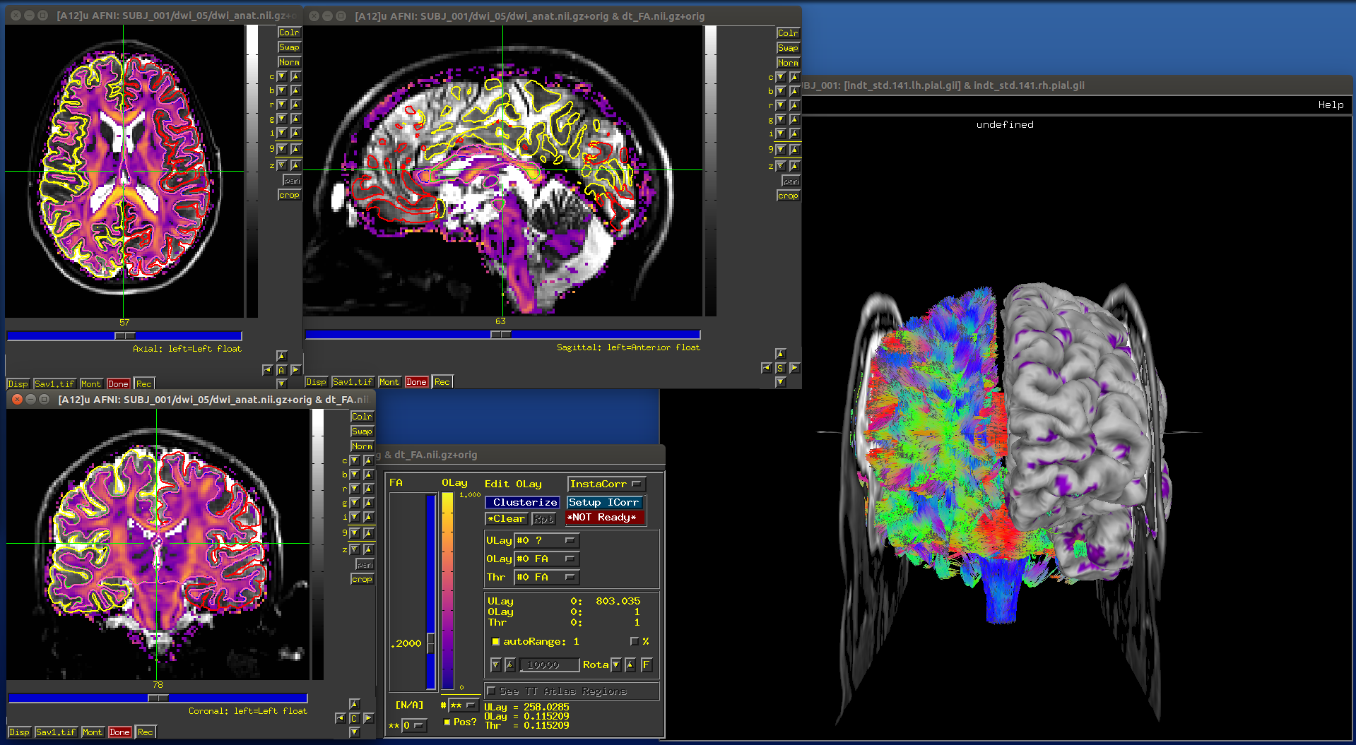
|
Viewing AFNI and SUMA talking together to display lots of structural data. The overlay in AFNI is the FA map thresholded at FA>0.2. |
Note
This is just the tip of the ice berg in terms of AFNI+SUMA viewing of structure, combining data and interactively viewing it. Please do download the the FATCAT Demo examples (again, see HERE), and check out the processing scripts there for more.