12.12.5. Using 2dcat

Introduction

Download script tarball: auto_2dcat.tgz

Open the tarball using tar -xf auto_2dcat.tgz to get the following scripts in your directory: tut_auto_2dcat_0.tcsh, tut_auto_2dcat_1.tcsh, tut_auto_2dcat_2.tcsh.

Download script: tut_auto_2dcat_0.tcsh

2dcat is an “image concatenation” program. This is a very useful supplementary tool for glueing existing images together to make arrays with separating lines, as well other features. It combines quite usefully with @chauffeur_afni, for example to concatenate similar images across a data set.

We present some examples of auto-image making with 2dcat using data that should be available in (modern) AFNI binary distributions, the *_SSW.nii.gz template targets for @SSwarper. Each of these dsets has multiple bricks. We provide examples:

• combining multiple views and slices of the same dataset

• adjoining similar views across separate datasets

and more.

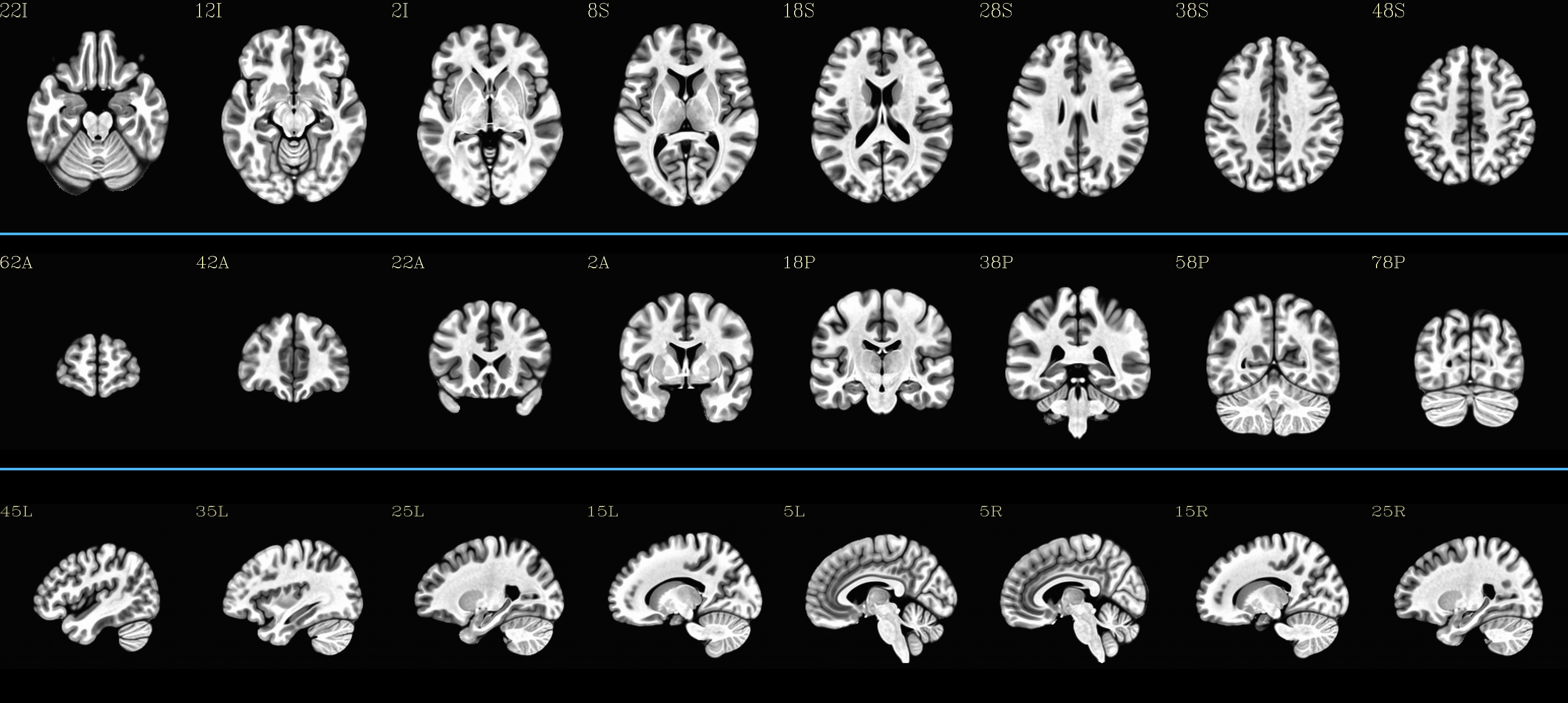
Each short script creates a subdirectory (“QC_2dcat*”) for the both the individual, intermediate images and the final concatenated matrix of images.

Ex. 0: Combine images subject- and slice-wise

Variables have been defined so that one should be able to adapt these scripts by changing the just file name(s) in the uppermost input section.

Definitions at top of script:

- show code y/n -

#!/bin/tcsh


# AFNI tutorial: auto-image-making example "0" using 2dcat (and
#                @chauffeur_afni)
#
# + last update: Feb 21, 2020
#   - name 'imcat' deprecated in favor of '2dcat'
#
##########################################################################
#
# Here, the program 2dcat concatenates (= glue together) images made
# with @chauffeur_afni.
#
# This script is meant to be run in a directory containing the
# "*_SSW.nii.gz" reference dsets (e.g., copied from "abin/" directory).
#
# We use the "*_SSW.nii.gz" reference templates distributed in AFNI.
# These dsets are used as reference volumes for @SSwarper (the
# combo-tool for performing nonlinear registration and skull stripping
# insieme).  Each of these dsets has multiple volumes (5).
#
# By changing the list of files given to "$istr", this script can be
# directly adapted to other cases.
#
# =====================================================================

set here  = $PWD                        # for path; trivial, could be changed

set istr  = "SSW"                       # string for choosing NIFTI files
set ilist = `\ls *${istr}.nii.gz`       # get list of NIFTIs to imagize
set Ndset = $#ilist                     # number of dsets in list

set lcol  = ( 255 255 255 )             # RGB line color bt image panels
set odir  = ${here}/QC_2dcat_00         # output dir for images

\mkdir -p ${odir}                       # make output dir

Use @chauffeur_afni to make individual images

Each @chauffeur_afni execution creates a set of sagittal, axial and coronal images; each image output by chauffeur here is an 8x1 montage. These will later be glued together.

set allbase = ()

foreach ff ( $ilist )

    set ibase   = `3dinfo -prefix_noext "${ff}"`  # base name of vol
    set allbase = ( $allbase $ibase )             # list of all base names

    # Make a montage of the zeroth brick of each dset
    @chauffeur_afni                                                   \
        -ulay       "${ff}[0]"                                        \
        -prefix     ${odir}/img0_${ibase}                             \
        -set_dicom_xyz   5 18 18                                      \
        -delta_slices   10 20 10                                      \
        -set_xhairs     OFF                                           \
        -montx 8 -monty 1                                             \
        -label_mode 1 -label_size 3                                   \
        -do_clean
end

Use 2dcat to concatenate sliceviews for each subj

First example of using 2dcat on a set of datasets: for each dset, concatenate different slice views (sagittal, coronal and axial) of a single volume.

This example requires having the *_SSW.nii.gz template targets copied into the present working directory. Alternatively, one could just include the path to them in the glob at the top of the script (e.g., set ivol  = `\ls ~/abin/*${istr}.nii.gz`)

# Just the "gap color" between glued-together images
set lcol  = ( 66 184 254 )

# For each volume, concatenate images across all 3 sliceviews.  The
# order of contanenation will be that of globbing; could be specified
# in different ways, too.
foreach ff ( $allbase )
    2dcat                                                             \
        -gap     5                                                    \
        -gap_col ${lcol}                                              \
        -nx 1                                                         \
        -ny 3                                                         \
        -prefix $odir/ALL_subj_${ff}.jpg                              \
        ${odir}/img0_*${ff}*
end

Combined sliceviews for each subject
HaskinsPeds_NL_template1.0_SSW:
MNI152_2009_template_SSW:
TT_N27_SSW:

Use 2dcat to concatenate subjs for each sliceview

Second example of using 2dcat on a set of datasets: for each slice view, show the dset at the same (x, y, z) location.

# Just the "gap color" between glued-together images
set lcol  = ( 255 152 11 )

# For each sliceview, concatenate images across all vols
foreach ss ( "sag" "cor" "axi" )
    2dcat                                                             \
        -gap     5                                                    \
        -gap_col ${lcol}                                              \
        -nx 1                                                         \
        -ny ${Ndset}                                                  \
        -prefix $odir/ALL_${istr}_sview_${ss}.jpg                     \
        ${odir}/img0_*${ss}*
end

# ---------------------------------------------------------------------

echo "++ DONE!"

# All fine
exit 0

Combined subjects for each sliceview
sagittal views:
coronal views:
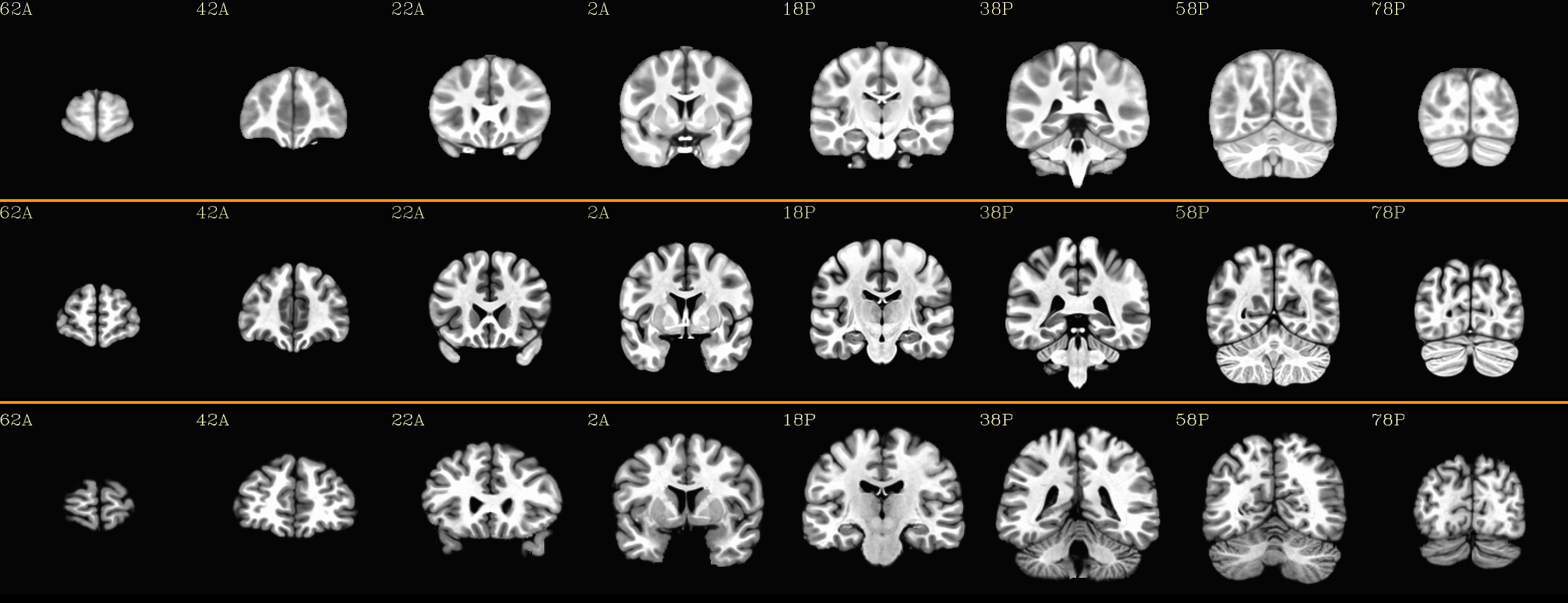
axial views:

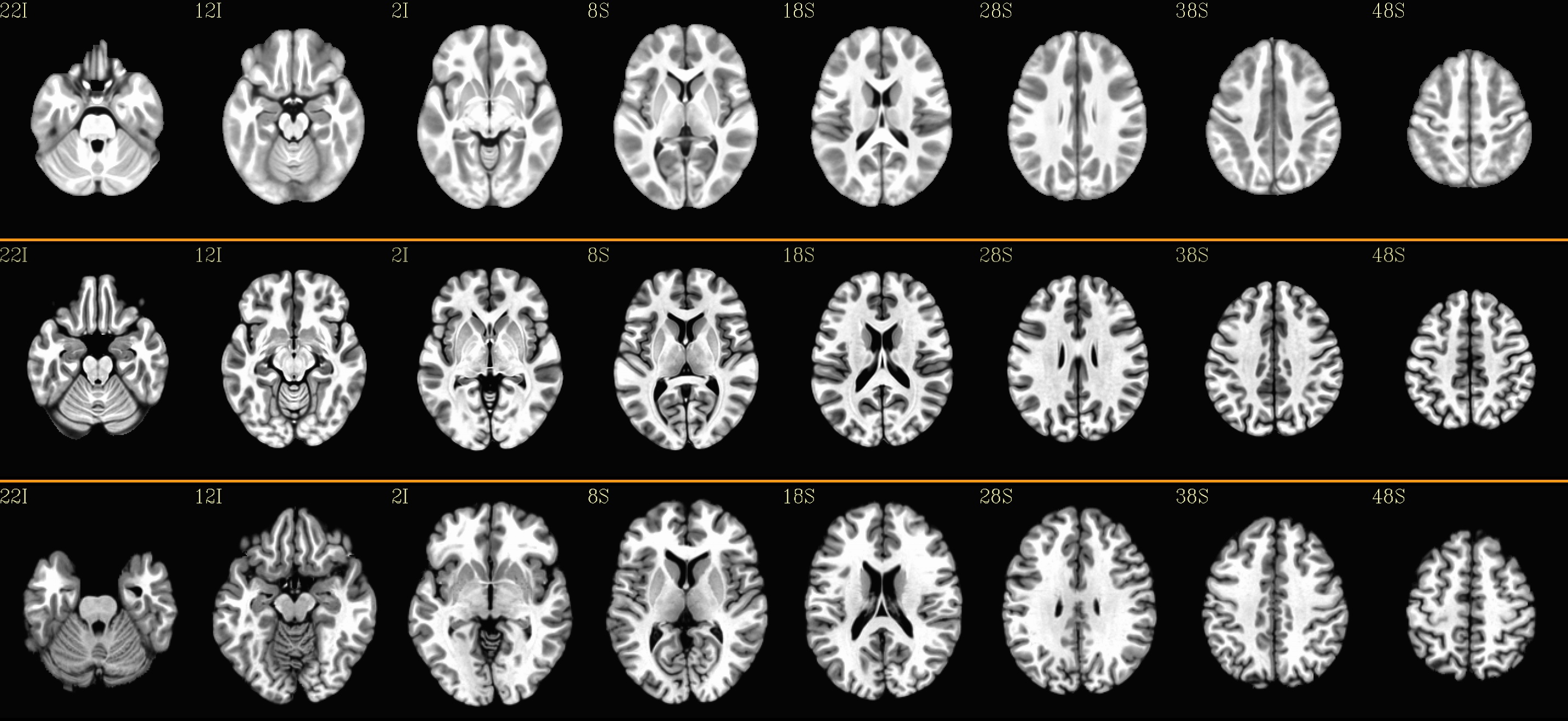
Ex. 1: Combine subbrick images of a 4D dset

Download script: tut_auto_2dcat_1.tcsh

Make a set of sagittal, axial and coronal images; these will later be glued together. Here, we are make a set of images per volume in a 4D dset.

Definitions at top of script:

- show code y/n -

#!/bin/tcsh


# AFNI tutorial: auto-image-making example "1" using 2dcat (and
#                @chauffeur_afni)
#
# + last update: Feb 21, 2020
#   - name 'imcat' deprecated in favor of '2dcat'
#
##########################################################################
#
# Here, the program 2dcat concatenates (= glue together) images made
# with @chauffeur_afni.
#
# Another example using one of the "*_SSW.nii.gz" reference templates
# distributed in AFNI.  Here, we view multiple subbricks of the dset.
#
# By changing the volume specified with "$ivol", this script can be
# directly adapted to other cases.
#
# =====================================================================

set here  = $PWD                            # for path; could be changed

set ivol  = MNI152_2009_template_SSW.nii.gz         # volume de choix
set ibase = `3dinfo -prefix_noext "${ivol}"`        # base name of vol
set nv    = `3dinfo -nv "${ivol}"`                  # number of vols
set imax  = `3dinfo -nvi "${ivol}"`                 # max index

set lcol  = ( 0 204 0 )                 # RGB line color bt image panels
set odir  = ${here}/QC_2dcat_01         # output dir for images

\mkdir -p ${odir}

Use @chauffeur_afni to make individual images

foreach ii ( `seq 0 1 ${imax}` )

    # zeropadded numbers, nicer to use in case we have a lot of images
    set iii = `printf "%03d" ${ii}`

    # This if-condition is a sidestep: we have two categories of data
    # in the input volume, masks and dsets, with very different
    # pertinent ranges, so we account for that here.
    if ( ${ii} > 2 ) then
        set UMIN = "0"
        set UMAX = "1"
    else
        set UMIN = "2%"
        set UMAX = "98%"
    endif

    @chauffeur_afni                                                   \
        -ulay       "${ivol}[$ii]"                                    \
        -ulay_range "$UMIN" "$UMAX"                                   \
        -prefix     ${odir}/${ibase}_${iii}                           \
        -set_dicom_xyz   2 18 18                                      \
        -delta_slices   25 25 25                                      \
        -set_xhairs     OFF                                           \
        -montx 1 -monty 1                                             \
        -label_mode 1 -label_size 3                                   \
        -do_clean
end

Use 2dcat to concatenate images

Combine the individual images from above into a matrix of images. Here we have three rows (i.e., three images along y-axis: one for sagittal, axial and coronal), and the number of columns is equal to the number of volumes in the 4D dset.

# concatenate 3 sliceviews, for as many volumes as are in the dset
2dcat                                                                 \
    -echo_edu                                                         \
    -gap 5                                                            \
    -gap_col ${lcol}                                                  \
    -nx ${nv}                                                         \
    -ny 3                                                             \
    -prefix $odir/ALL_vol_${ibase}.jpg                                \
    $odir/${ibase}*sag* $odir/${ibase}*cor* $odir/${ibase}*axi*

# ---------------------------------------------------------------------

echo "++ DONE!"

# All fine
exit 0

Ex. 1: Each subject & all sliceviews
MNI152_2009_template_SSW:

Ex. 2: Combine (stats) images from many subj

Download script: tut_auto_2dcat_2.tcsh

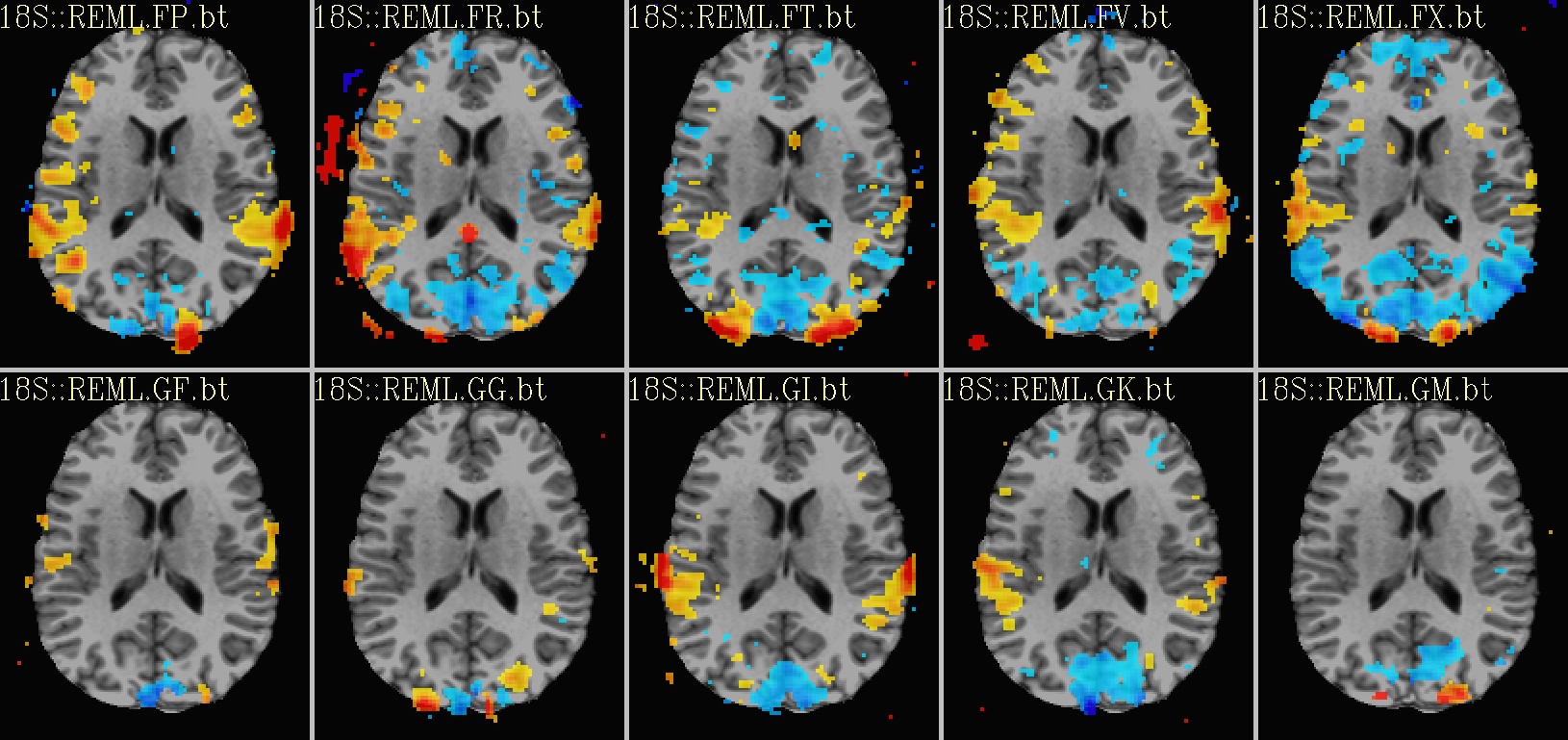
Here we present a nice way to make a summary of similar images across a group of subjects. In this case, we use a set of individual modeling results: we threshold based on a statistical criterion (voxelwise p<0.001, two-sided) and show the effect estimates (beta coefficients).

We can apply the typical hard thresholding, where everything in subthreshold voxels is hidden. Or, we can use a more modern alpha thresholding, whereby subthreshold voxels are merely made increasingly transparent as their values are further below threshold.

Definitions at top of script:

- show code y/n -

#!/bin/tcsh


# AFNI tutorial: auto-image-making example "2" using 2dcat (and
#                @chauffeur_afni)
#
# + last update: Feb 21, 2020
#   - name 'imcat' deprecated in favor of '2dcat'
#
##########################################################################
#
# This example shows one way to look at individual statistical results
# across a group.
#
# This tcsh script is meant to be run in the following directory of
# the AFNI Bootcamp demo data:
#     AFNI_data6/group_results
# using the REML* volumes there.
#
# By changing the the list of files given to "${ilist}", this can be
# directly adapted to other cases.  Depending on how you unpacked your
# Bootcamp data, you might need to adjust the "${idir}" variable, too.
#
# =====================================================================

set here  = $PWD                          # for path; trivial, could be changed

set istr   = "REML"                       # string for choosing vol dsets
set idir   = "~/AFNI_data6/group_results" # location of files (at least for me)
set ilist  = `\ls ${idir}/${istr}*HEAD`   # get list of dsets to imagize
set imask  = "${idir}/mask+tlrc.HEAD"     # WB mask for this 'group'
set ianat  = "${idir}/FT_anat+tlrc.HEAD"  # anat vol, use as ulay

set lcol  = ( 192 192 192 )               # RGB line color bt image panels
set odir  = ${here}/QC_2dcat_02           # output dir for images

\mkdir -p ${odir}

Use @chauffeur_afni to make individual images

set allbase = ()

foreach ff ( ${ilist} )
    # base name of vol, and make a list of all prefixes for later
    set ibase   = `3dinfo -prefix_noext "${ff}"`
    set allbase = ( ${allbase} ${ibase} )

    ### Make a montage of the zeroth brick of each image.
    # Some fun-ness here: part of each file's name is added to the
    # label string shown in each panel.
    # Note: these olay datasets are unclustered and unmasked.
    @chauffeur_afni                                                   \
        -ulay       ${ianat}                                          \
        -ulay_range "2%" "130%"                                       \
        -olay       ${ff}                                             \
        -set_subbricks -1 0 1                                         \
        -func_range 3                                                 \
        -thr_olay_p2stat 0.001                                        \
        -thr_olay_pside  bisided                                      \
        -cbar    Reds_and_Blues_Inv                                   \
        -olay_alpha  Yes                                              \
        -olay_boxed  Yes                                              \
        -opacity 7                                                    \
        -prefix     ${odir}/img0_alpha_${ibase}                       \
        -montx 1 -monty 1                                             \
        -set_dicom_xyz  5 18 18                                       \
        -set_xhairs     OFF                                           \
        -label_string "::${ibase}"                                    \
        -label_mode 1 -label_size 3                                   \
        -do_clean

    # same images as above, but with hard thresholding
    @chauffeur_afni                                                   \
        -ulay       ${ianat}                                          \
        -ulay_range "2%" "130%"                                       \
        -olay       ${ff}                                             \
        -set_subbricks -1 0 1                                         \
        -func_range 3                                                 \
        -thr_olay_p2stat 0.001                                        \
        -thr_olay_pside  bisided                                      \
        -cbar    Reds_and_Blues_Inv                                   \
        -opacity 7                                                    \
        -prefix     ${odir}/img0_hthr_${ibase}                        \
        -montx 1 -monty 1                                             \
        -set_dicom_xyz  5 18 18                                       \
        -set_xhairs     OFF                                           \
        -label_string "::${ibase}"                                    \
        -label_mode 1 -label_size 3                                   \
        -do_clean

end

Use 2dcat to concatenate images

Combine the individual images from above into a matrix of images. Here we combine similar slice views. Note how we end up having a nice summary of subject modeling results across the group.

Scripting note : Note that here the nx and ny values are hardcoded in, but they needn’t be, so this script could be more flexible to match adding/subtracting subjects. Fancier things can be done– feel free to ask/discuss/recommend suggestions.

foreach ss ( "sag" "cor" "axi" )
    # Combine alpha-thresholded images
    2dcat                                                             \
        -echo_edu                                                     \
        -gap 5                                                        \
        -gap_col ${lcol}                                              \
        -nx 5                                                         \
        -ny 2                                                         \
        -prefix ${odir}/ALL_alpha_${istr}_sview_${ss}.jpg             \
        ${odir}/img0_alpha*${ss}*

    # Combine hard-thresholded images
    2dcat                                                             \
        -echo_edu                                                     \
        -gap 5                                                        \
        -gap_col ${lcol}                                              \
        -nx 5                                                         \
        -ny 2                                                         \
        -prefix ${odir}/ALL_hthr_${istr}_sview_${ss}.jpg              \
        ${odir}/img0_hthr_*${ss}*

end

# ---------------------------------------------------------------------

echo "++ DONE!"

# All fine
exit 0

Ex. 2: One stat slice across subjects: alpha+boxed thresholding
sagittal views:
coronal views:
axial views:

Ex. 2: One stat slice across subjects: hard thresholding
sagittal views:
coronal views:
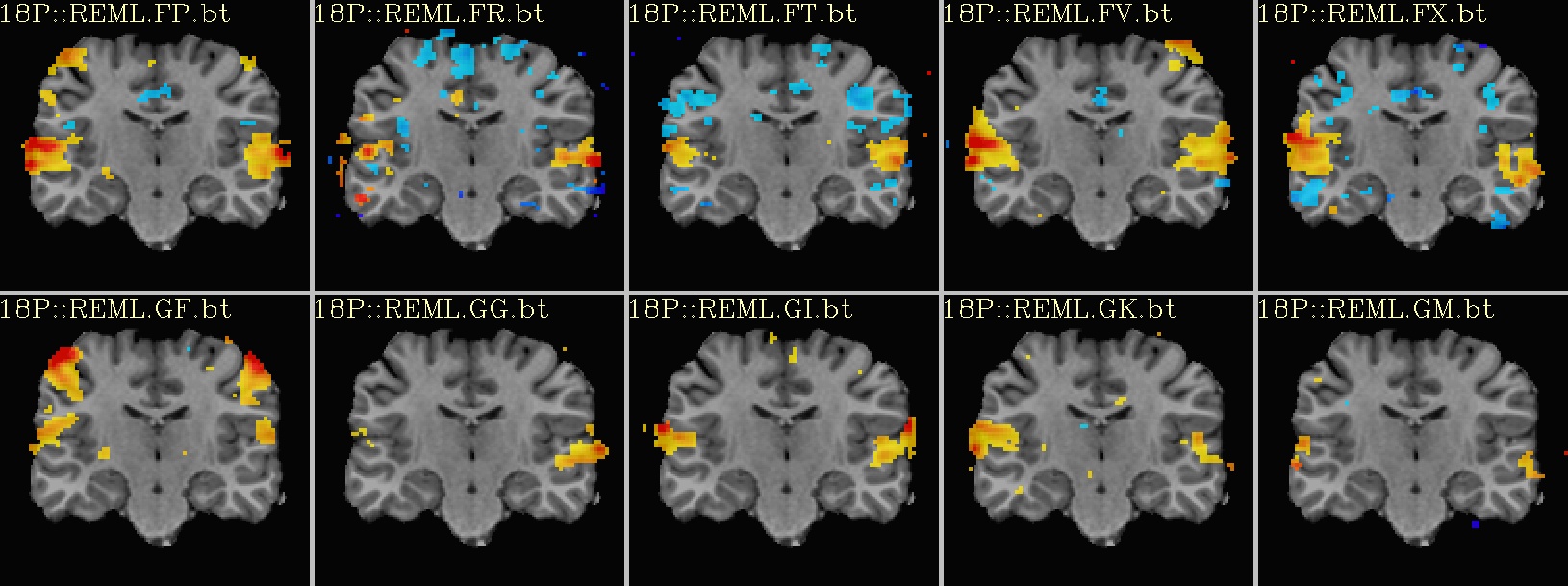
axial views: