12.12.2. Using @chauffeur_afni
Introduction
Download script: tut_auto_@chauffeur_afni.tcsh
@chauffeur_afni creates+saves images (JPG, PNG, etc.) or movies
(MP3, etc.) of volumetric data sets. The primary purpose of this
program is to help users look at their data as and after they process
it.
It can be used to view either:
multiple slices within a single 3D volume
a single slice across a multiple volumes in a 4D dataset.
Image files are produced in sets of 3: one each of axial, coronal and sagittal slices. One can view either olay+ulay combinations, or just a ulay dset.
This program works semi-magically by wrapping around a lot of the AFNI’s underlying “driving” capabilities and environment variables. The full list of these are provided in these fun documentation pages, provided for The Curious amongst you:
@chauffeur_afni embeds as much of that functionality as possible
(or as asked-for) with the convenience of command line options.
- Historical note:
This program was originally written for use within FATCAT fat_proc* tools tools (generalizing the visualization of
@snapshot_volreg). Thefat_proc*programs call@chauffeur_afniinternally, generating images at each step of the pipeline that can be reviewed later as a first pass evaluation of the data processing. This program drives a lot of the image-generating capability of HTML QC output ofafni_proc.py, too.
Examples, and how to run them
For the @chauffeur_afni image-making examples below, we use data
of the AFNI_data6/afni/ directory of the freely available AFNI
Bootcamp demo sets (see here if you don’t have it
yet).
The code snippets can all be run in a single (tcsh) script file
(provided above)– the variable names are consistent throughout the
page, starting from the initial definitions. Just save the script in
your AFNI_data6/afni/ directory.
A few supplementary volumes/text files will be generated and added to
the directory. The images themselves are put into a subdirectory
called QC/ that is created. Several of the examples include
thresholding statistical output data sets, and therefore include
running additional AFNI programs like 3dClusterize, etc. And all
at no extra charge!
Some of the examples build on each other. Not every style of image is the most recommended, but they are chosen to demonstrate a lot of options, as well as relative benefits of some choices compared to others.
To toggle between images: open each of the images you want to move
between/among in a separate browser tab (e.g., middle mouse click on
it), and then move between tabs (e.g., Ctrl + Tab and Ctrl
+ Shift + Tab).
Top of script: The following commands use almost no variable
syntax—in fact, just the output prefix ${opref} in each case.
The displayed syntax for setting this variable is tcsh, but you
could adjust any of these to be another shell if you wish. For
example, in bash or zsh, the first variable setting would be
opref=QC/ca000_anat_def. The only other overhead that the script
does is making the output directory, which is done with \mkdir -p
QC (shell independent).
#!/bin/tcsh
# AFNI tutorial: series of examples of automatic image-making in AFNI.
#
# + last update: Oct 21, 2021
#
##########################################################################
# This tcsh script is meant to be run in the following directory of
# the AFNI Bootcamp demo data:
# AFNI_data6/afni
#
# ----------------------------------------------------------------------
# make output dir for all images
\mkdir -p
QC
Ex. 0: Simple underlay viewing
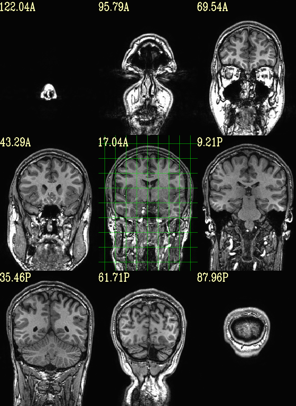
Simply view the (non-skullstripped) anatomical volume as an underlay by itself. Might be useful to check for artifact, coverage, etc. The full crosshair grid shows where slices are taken from, and might be useful for seeing the relative alignment/axialization of the brain.
Unless specified otherwise, the ulay black/white mapping is to 0%/98% of voxels in the whole volume. The AFNI GUI uses 2%/98% of slicewise percentiles by default, but since default viewing here is montage-based, volumewise is implemented by default for consistency across both the individual view-plane montage as well as across three view-planes that are created per command execution.
set opref = QC/ca000_anat_def

@chauffeur_afni                                                       \
    -ulay         anat+orig.HEAD                                      \
    -prefix       ${opref}                                            \
    -set_xhairs   MULTI                                               \
    -montx 3 -monty 3                                                 \
    -label_mode 1 -label_size 4
Example 0 |
|
|---|---|

|
|

|
Ex. 1: Moving/selecting view slices
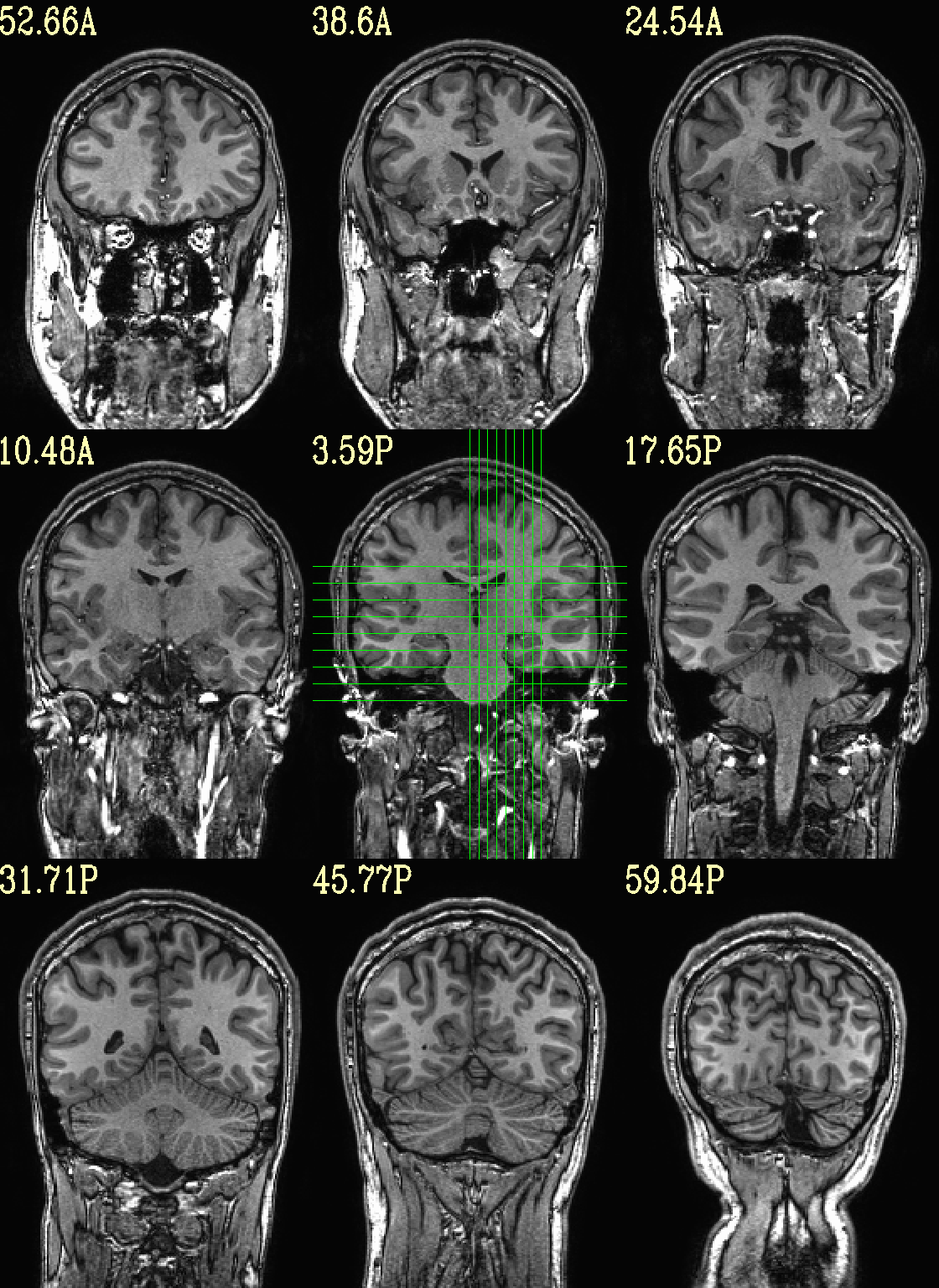
By default, the image slices are set as follows: if there are N total images in the montage, place N along each axis spaced as evenly as possible (as done in the previous example).
However, users can specify either the (x, y, z) or (i, j, k) location of the central slice, as well as spacing between each of the N slices (the “delta” number of rows/columns between image slices). In this example the central image is placed at the location (x, y, z) = (-10 4 3), and different slice spacing is specified along different axes.
set opref = QC/ca001_anat_mv_slices

@chauffeur_afni                                                       \
    -ulay           anat+orig.HEAD                                    \
    -prefix         ${opref}                                          \
    -set_dicom_xyz  -20 4 3                                           \
    -delta_slices   5 15 10                                           \
    -set_xhairs     MULTI                                             \
    -montx 3 -monty 3                                                 \
    -label_mode 1 -label_size 4
Example 1 |
|
|---|---|

|
|

|
Ex. 2: Underlay and overlay viewing (mask example)
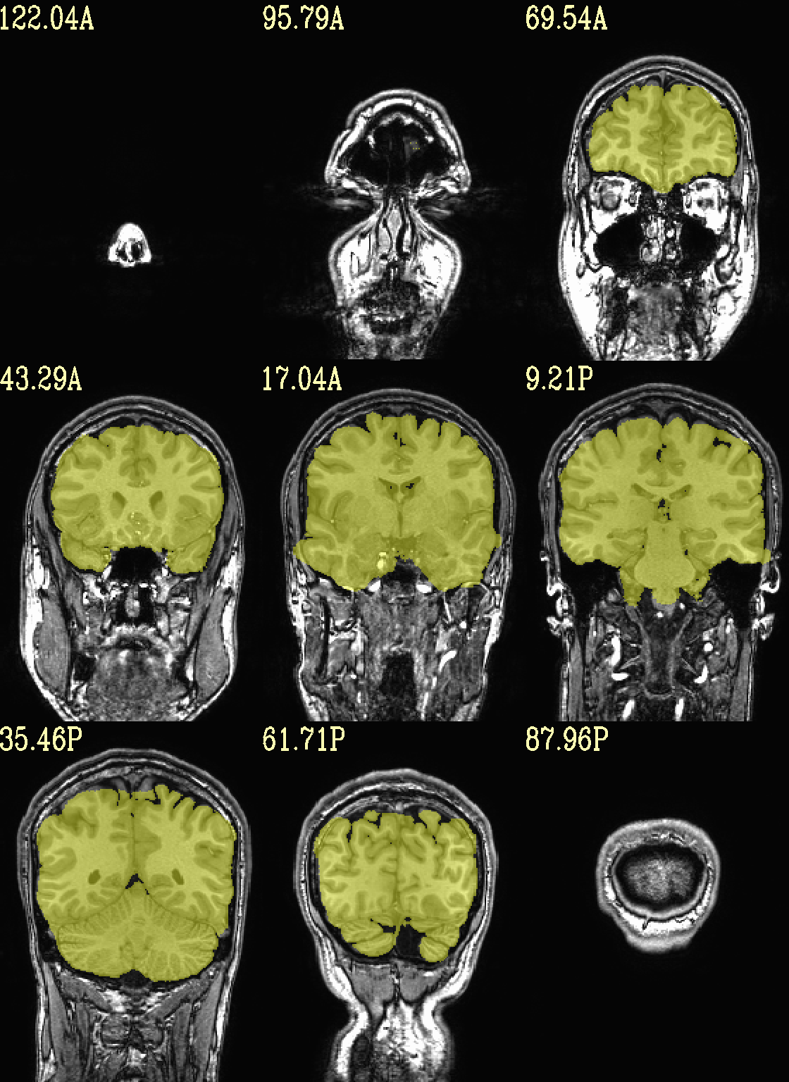
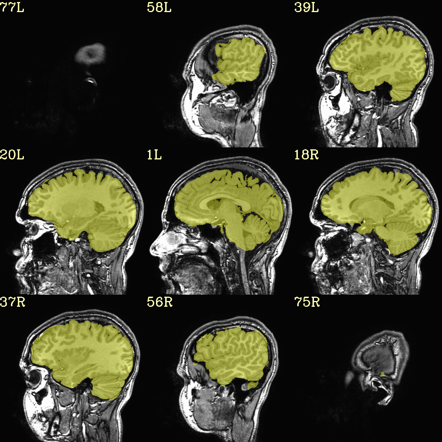
(Going back to evenly spread slices…) Add an overlay with some transparency to the previous anatomical– here, a binary mask of the skullstripped volume to check the quality of the skullstripping results. The olay color comes from the max of the default colorbar (‘Plasma’).
The crosshairs have also been turned off.
# binarize the skullstripped anatomical, if not already done
if ( ! -e anat_mask.nii.gz ) then
    3dcalc                                                            \
        -a       strip+orig.HEAD                                      \
        -expr    'step(a)'                                            \
        -prefix  anat_mask.nii.gz
endif

set opref = QC/ca002_anat_w_mask

@chauffeur_afni                                                       \
    -ulay         anat+orig.HEAD                                      \
    -olay         anat_mask.nii.gz                                    \
    -opacity      4                                                   \
    -prefix       ${opref}                                            \
    -set_xhairs   OFF                                                 \
    -montx 3 -monty 3                                                 \
    -label_mode 1 -label_size 4
Example 2 |
|
|---|---|

|
|
|
Ex. 3: Focus box to select view slices
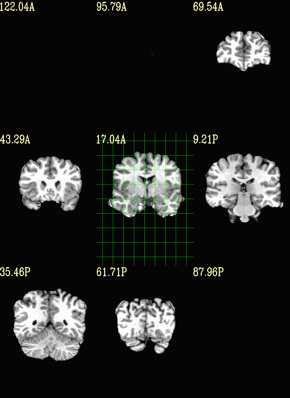
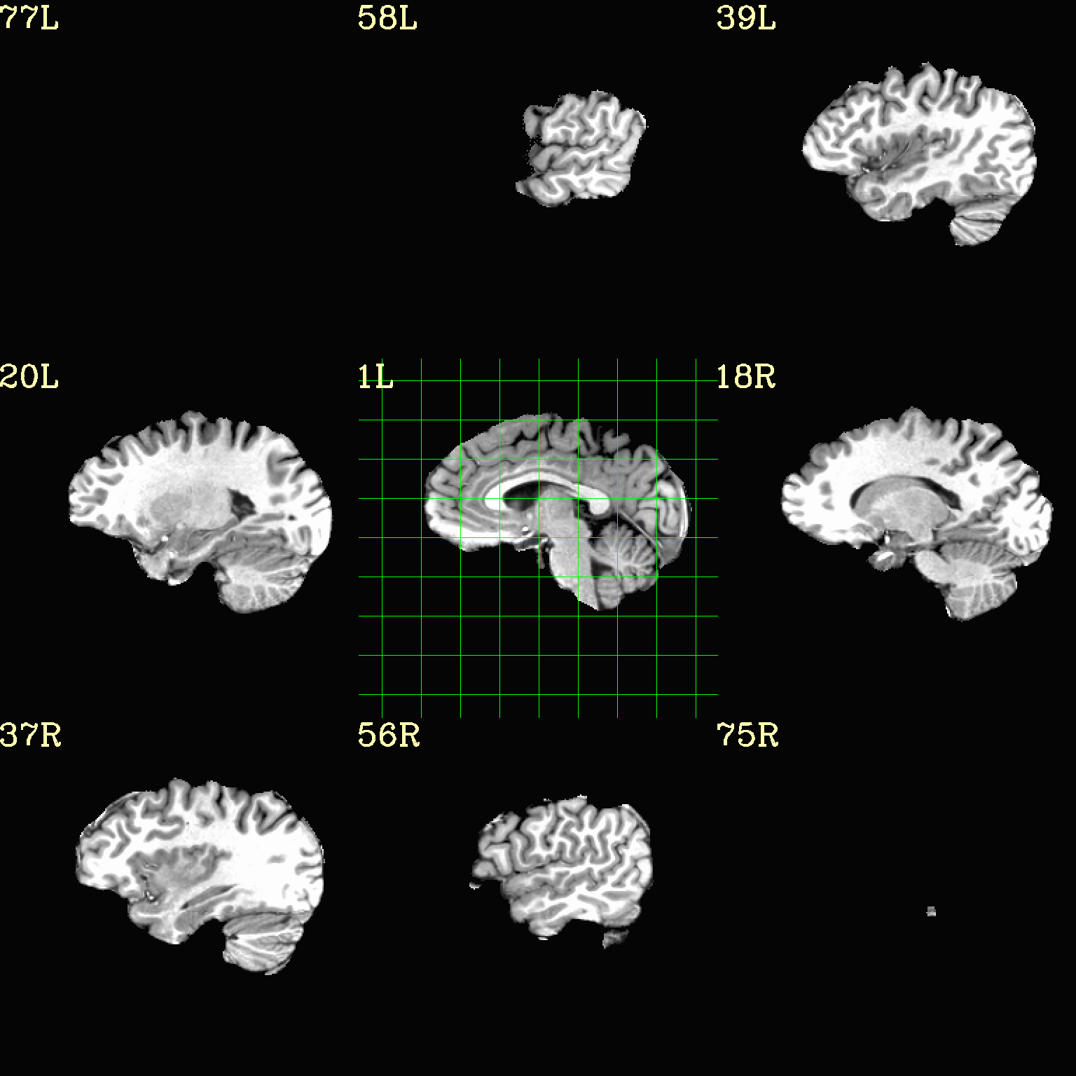
Sometimes there is lots of empty space in a FOV; so just viewing the default, even spread of slices can leave lots of wasted empty space such as here:
set opref = QC/ca003a_anat_w_space

@chauffeur_afni                                                       \
    -ulay         strip+orig.HEAD                                     \
    -prefix       ${opref}                                            \
    -set_xhairs   MULTI                                               \
    -montx 3 -monty 3                                                 \
    -label_mode 1 -label_size 4
Example 3a |
|
|---|---|

|
|
|
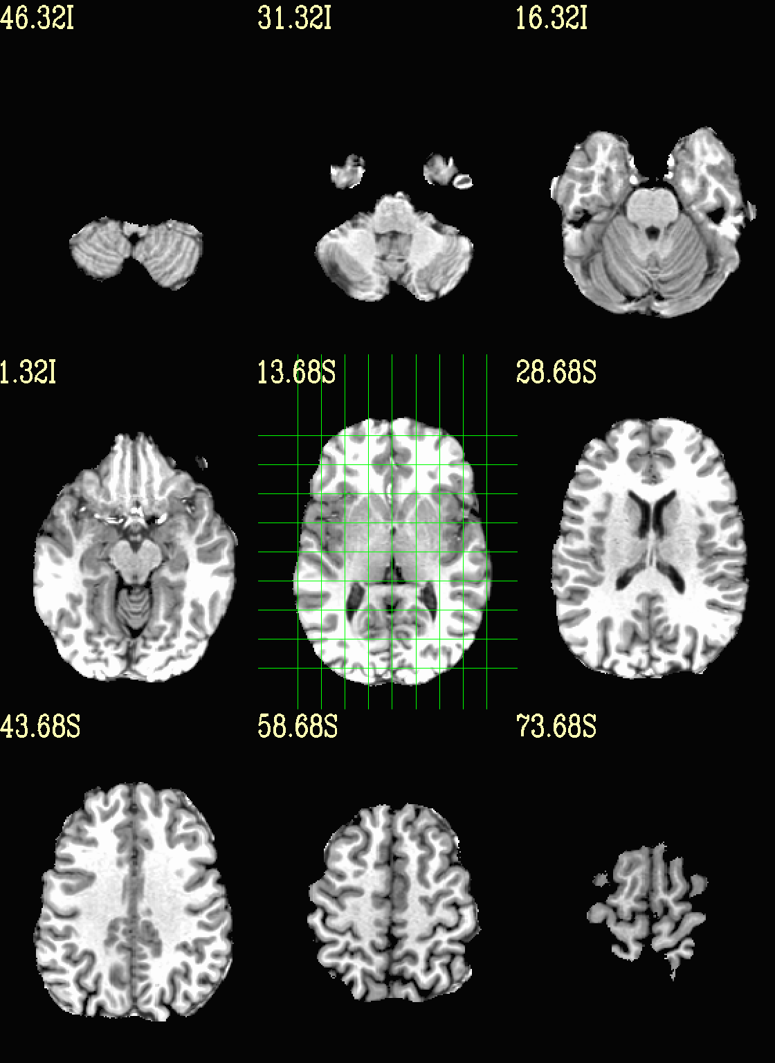
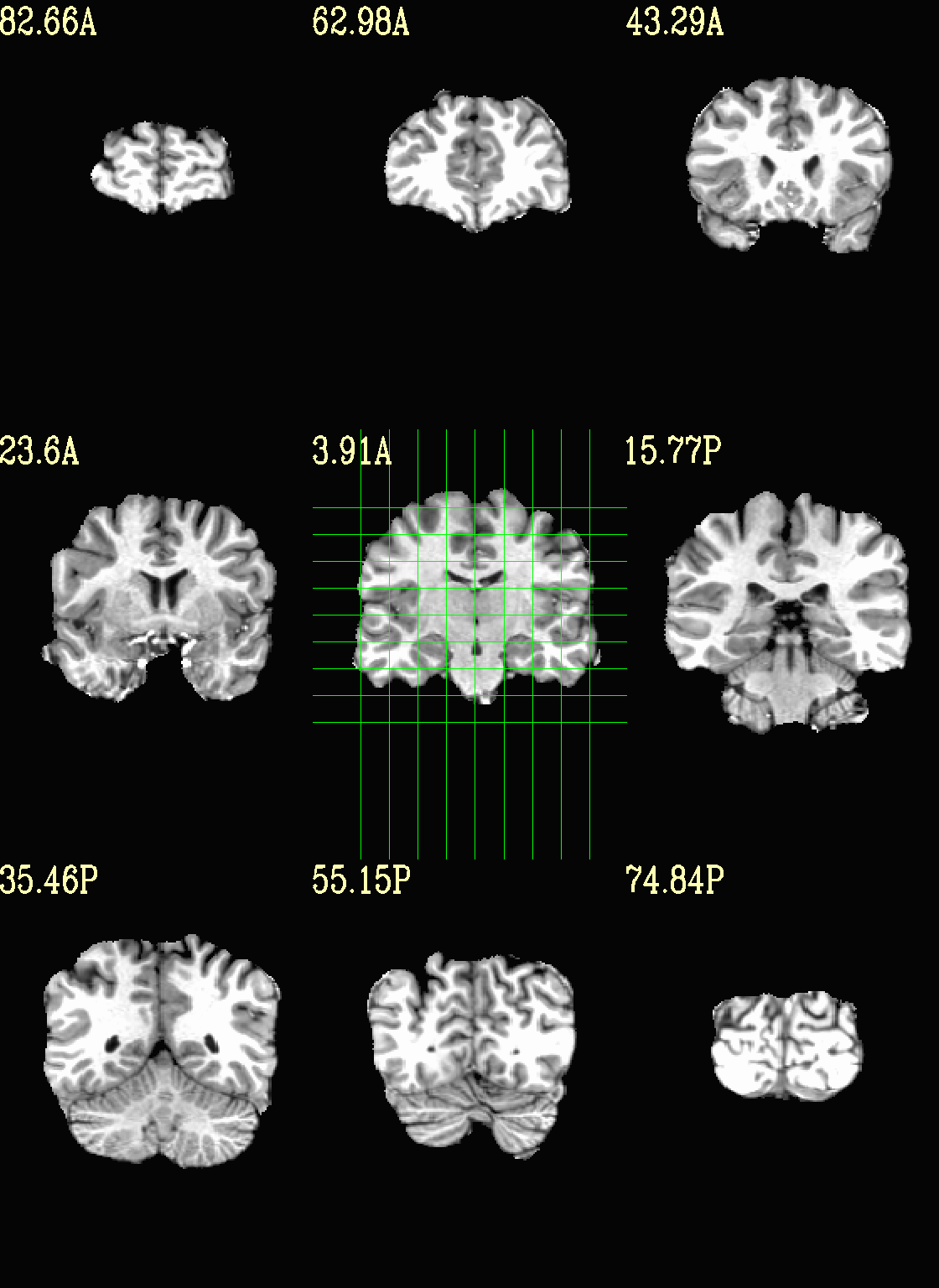
To avoid this without needed to autobox a dset or anything, we can use a dset or keyword to focus the slices within which viewing occurs, and then have the program make the evenly spaced montage within that restricted view.
In the following case, we use a keyword to use the underlay as a reference, which will be internally autoboxed before viewing (and this can be done when an overlay is present, or using the overlay, or using a totally different dataset). This is often extremely useful if there is a lot of empty space:
set opref = QC/ca003b_anat_w_space

@chauffeur_afni                                                       \
    -ulay              strip+orig.HEAD                                \
    -box_focus_slices  AMASK_FOCUS_ULAY                               \
    -prefix            ${opref}                                       \
    -set_xhairs        MULTI                                          \
    -montx 3 -monty 3                                                 \
    -label_mode 1 -label_size 4
Example 3b |
|
|---|---|
|
|

|
Ex. 4: Overlay beta coefs and threshold with stats
Pretty standard “vanilla mode” of seeing thresholded statistic results of (task) FMRI modeling. In AFNI we strongly recommend viewing the effect estimate (“coef”, like the beta in a GLM, for example) as the olay, and using its associated statistic for voxelwise thresholding. The range of the functional data is “3”, since that might be a reasonable max/upper response value for this FMRI data that has been scaled to meaningful BOLD %signal change units; the colorbar is just the one that is default in AFNI GUI.
The threshold appropriate for this statistic was generated by
specifying a p-value, and then using the program p2dsetstat to
read the header info for that volume and do the p-to-stat conversion.
In this example, we have to know that the coefficient of interest is
the [1] volume, and its stat is the [2] volume (later we can
use labels, instead).
Here, the underlay is just the skullstripped anatomical volume.
Note that the slice location is shown in each panel (in a manner agnostic to the dset’s orientation like RAI, LPI, SRA, etc.).
# determine voxelwise stat threshold, using p-to-statistic
# calculation
set sthr = `p2dsetstat                                                \
                -inset   "func_slim+orig.HEAD [2]"                    \
                -pval    0.001                                        \
                -bisided                                              \
                -quiet`

echo "++ The p-value 0.001 was convert to a stat value of: ${sthr}."

set opref = QC/ca004a_Vrel_coef_stat

@chauffeur_afni                                                       \
    -ulay             strip+orig.HEAD                                 \
    -olay             func_slim+orig.HEAD                             \
    -box_focus_slices AMASK_FOCUS_ULAY                                \
    -func_range       3                                               \
    -cbar             Spectrum:red_to_blue                            \
    -thr_olay         ${sthr}                                         \
    -set_subbricks    -1 1 2                                          \
    -opacity          5                                               \
    -prefix           ${opref}                                        \
    -set_xhairs       OFF                                             \
    -montx 3 -monty 3                                                 \
    -label_mode 1 -label_size 4
Example 4a |
|
|---|---|

|

|

|
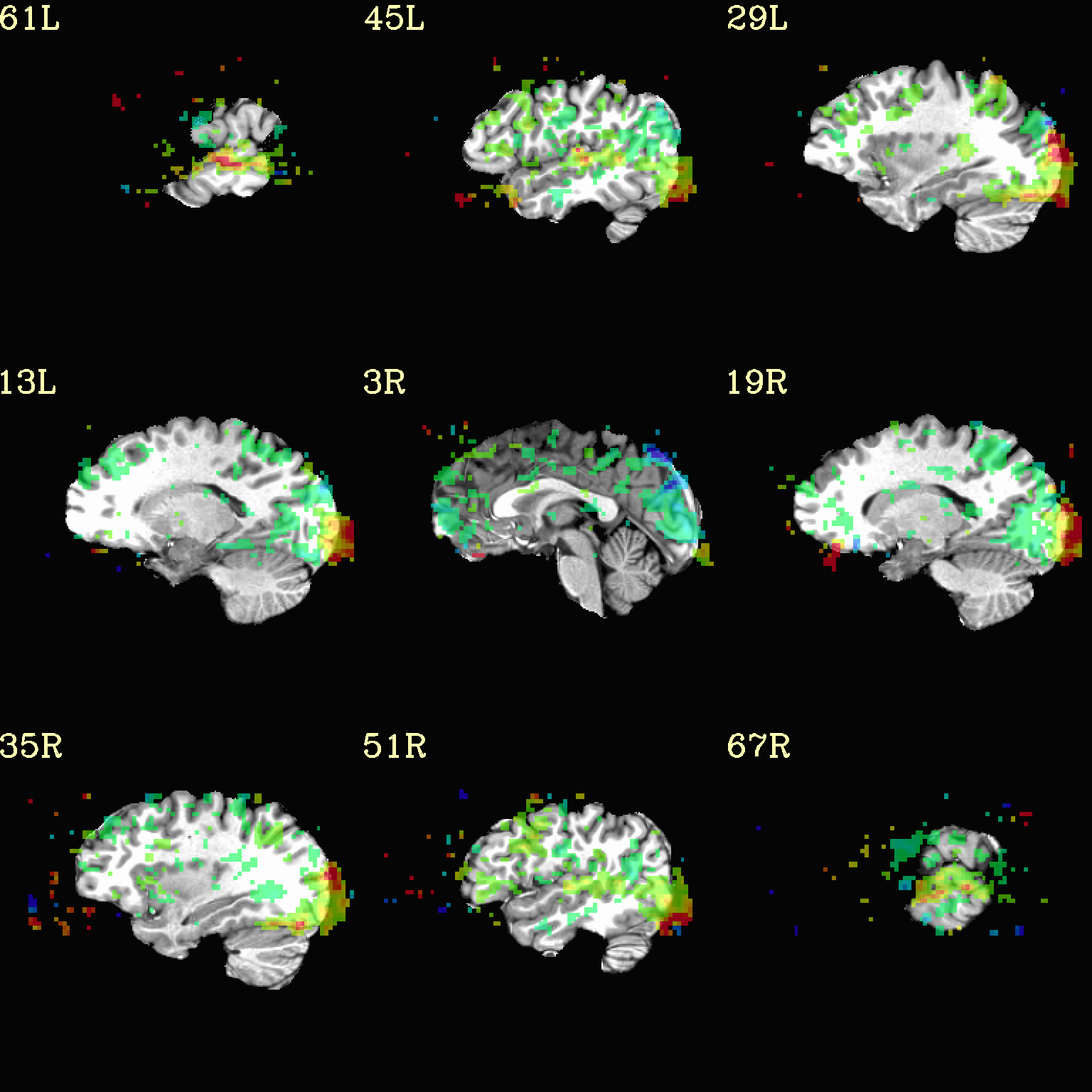
Now, let’s do that, just a little more conveniently with
@chauffeur_afni: use subbrick labels to refer to things (in
-set_subbricks ..), and have the p-to-stat conversion happen
internally (with -thr_olay_p2stat).
set opref = QC/ca004b_Vrel_coef_stat

@chauffeur_afni                                                       \
    -ulay             strip+orig.HEAD                                 \
    -olay             func_slim+orig.HEAD                             \
    -box_focus_slices AMASK_FOCUS_ULAY                                \
    -func_range       3                                               \
    -cbar             Spectrum:red_to_blue                            \
    -thr_olay_p2stat  0.001                                           \
    -thr_olay_pside   bisided                                         \
    -set_subbricks    -1 "Vrel#0_Coef" "Vrel#0_Tstat"                 \
    -opacity          5                                               \
    -prefix           ${opref}                                        \
    -set_xhairs       OFF                                             \
    -montx 3 -monty 3                                                 \
    -label_mode 1 -label_size 4
Example 4b |
|
|---|---|

|

|
|
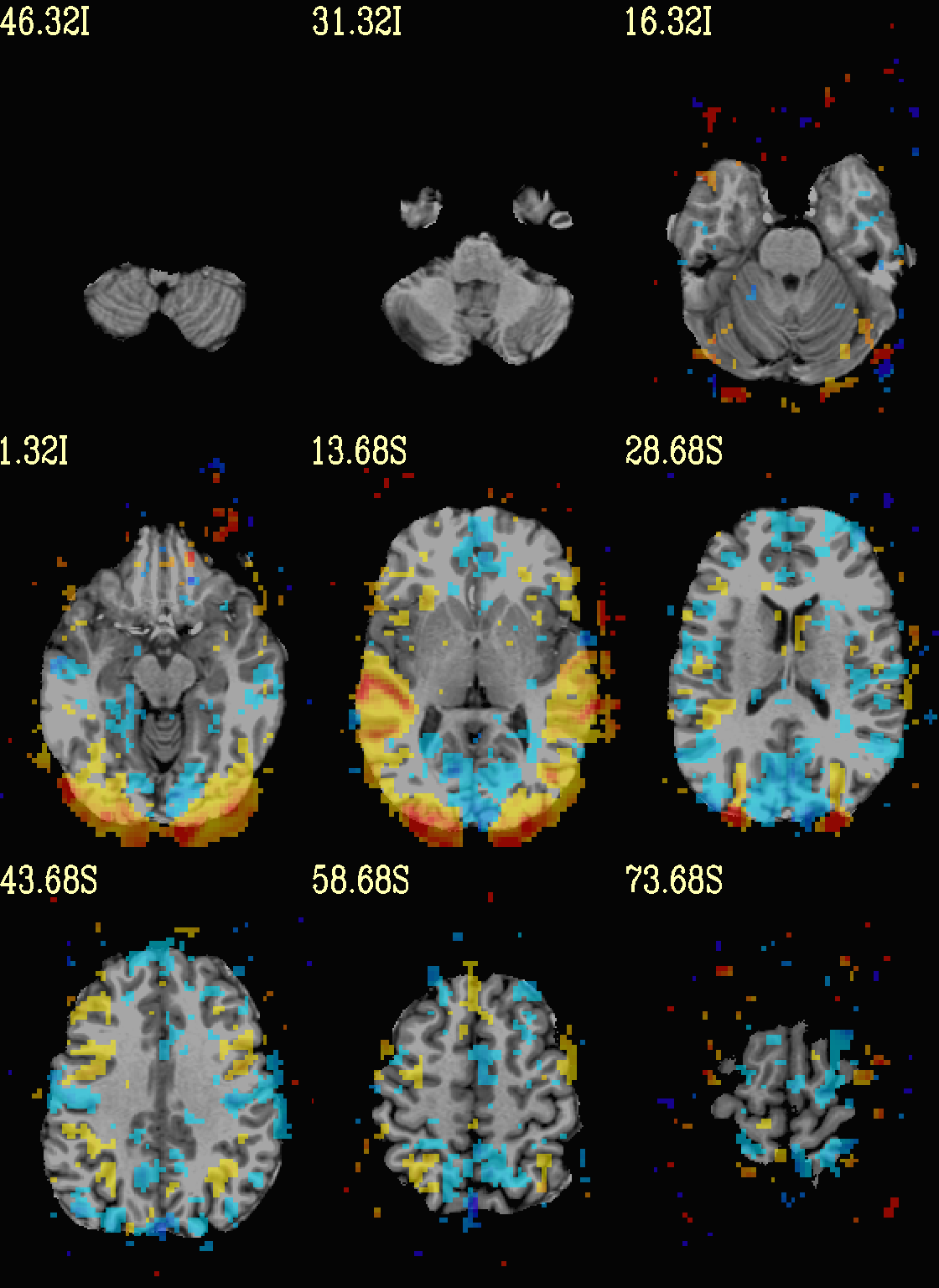
Finally, we can also tweak the colorbar for a bit of more clear
positive/negative affect separation (with -cbar ..).
Additionally, we might darken the underlay a bit by scaling its
brightness now, to make the overlay “pop” a little more visually (with
-ulay_range ..).
set opref = QC/ca004c_Vrel_coef_stat

@chauffeur_afni                                                       \
    -ulay             strip+orig.HEAD                                 \
    -ulay_range       0% 130%                                         \
    -olay             func_slim+orig.HEAD                             \
    -box_focus_slices AMASK_FOCUS_ULAY                                \
    -func_range       3                                               \
    -cbar             Reds_and_Blues_Inv                              \
    -thr_olay_p2stat  0.001                                           \
    -thr_olay_pside   bisided                                         \
    -set_subbricks    -1 "Vrel#0_Coef" "Vrel#0_Tstat"                 \
    -opacity          5                                               \
    -prefix           ${opref}                                        \
    -set_xhairs       OFF                                             \
    -montx 3 -monty 3                                                 \
    -label_mode 1 -label_size 4
Example 4c |
|
|---|---|
|

|

|
Ex. 5: Overlay beta coefs and threshold translucently with stats
Another take on thresholding: one without being so strict, and showing more of the data. For example, it might be quite informative to still see some of the “near misses” in the data.
One can soften the ON/OFF binarization of thresholding, by decreasing
the “alpha” level—or opacity—of sub-threshold voxels in a
continuous manner (-olay_alpha ..): either quadratically (used
here) or linearly (less steep decline in visibility). To still mostly
highlight the suprathreshold voxels, we can add a black-lined box
around them (with -olay_boxed Yes).
This is a really nice way to view modeling information, and is
utilized often in the QC HTML created by afni_proc.py (see
here).
set opref = QC/ca005a_Vrel_coef_stat

@chauffeur_afni                                                       \
    -ulay             strip+orig.HEAD                                 \
    -ulay_range       0% 130%                                         \
    -olay             func_slim+orig.HEAD                             \
    -box_focus_slices AMASK_FOCUS_ULAY                                \
    -func_range       3                                               \
    -cbar             Reds_and_Blues_Inv                              \
    -thr_olay_p2stat  0.001                                           \
    -thr_olay_pside   bisided                                         \
    -olay_alpha       Yes                                             \
    -olay_boxed       Yes                                             \
    -set_subbricks    -1 "Vrel#0_Coef" "Vrel#0_Tstat"                 \
    -opacity          5                                               \
    -prefix           ${opref}                                        \
    -set_xhairs       OFF                                             \
    -montx 3 -monty 3                                                 \
    -label_mode 1 -label_size 4
Example 5a |
|
|---|---|

|

|

|
Ex. 6: Overlay beta coefs, threshold with stats and clusterize
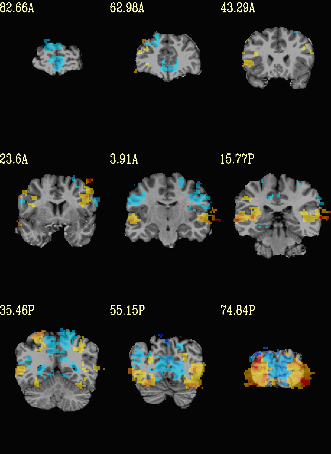
The previous examples were just thresholded voxelwise. This used
3dClusterize to add in cluster-volume thresholding to this;
the program generates both the effect estimate volume (“EE”) as well
as a map of the clusters (“map”, has a different integer per ROI,
sorted by size) produced by the dual thresholding. The clustersize of
200 voxels was just chosen arbitrarily (but could be calculated for
real data with 3dClustSim, for example).
Comment on ``3dClusterize`` usage: in most cases, you will have a mask to apply to the data being clustered, to either use in the command, or perhaps having already applied it to an intermediate version of the data. If you have a mask in the header of the stats file, then you can add an opt “-mask_from_hdr” to this command to read it directly from the header, similar to usage in the GUI.
The rest of the visualization aspects of the coefficient (beta, or effect estimate) volume here are pretty similar to the preceding.
3dClusterize                                                          \
    -overwrite                                                        \
    -echo_edu                                                         \
    -inset          func_slim+orig.HEAD                               \
    -ithr           "Vrel#0_Tstat"                                    \
    -idat           "Vrel#0_Coef"                                     \
    -bisided        "p=0.001"                                         \
    -NN             1                                                 \
    -clust_nvox     200                                               \
    -pref_map       clust_Vrel_map.nii.gz                             \
    -pref_dat       clust_Vrel_coef.nii.gz                            \
  >  clust_Vrel_report.1D

set opref = QC/ca006a_Vrel

@chauffeur_afni                                                       \
    -ulay              strip+orig.HEAD                                \
    -box_focus_slices  AMASK_FOCUS_ULAY                               \
    -olay              clust_Vrel_coef.nii.gz                         \
    -cbar              Reds_and_Blues_Inv                             \
    -ulay_range        0% 130%                                        \
    -func_range        3                                              \
    -opacity           5                                              \
    -prefix            ${opref}                                       \
    -set_xhairs        OFF                                            \
    -montx 3 -monty 3                                                 \
    -label_mode 1 -label_size 4
Example 6a |
|
|---|---|

|
|

|
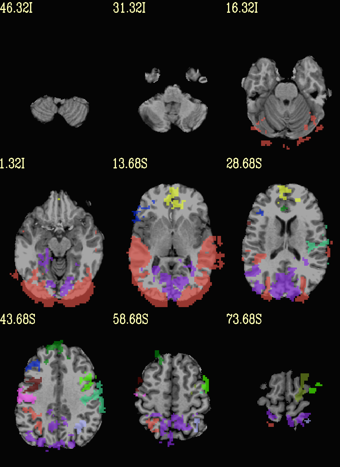
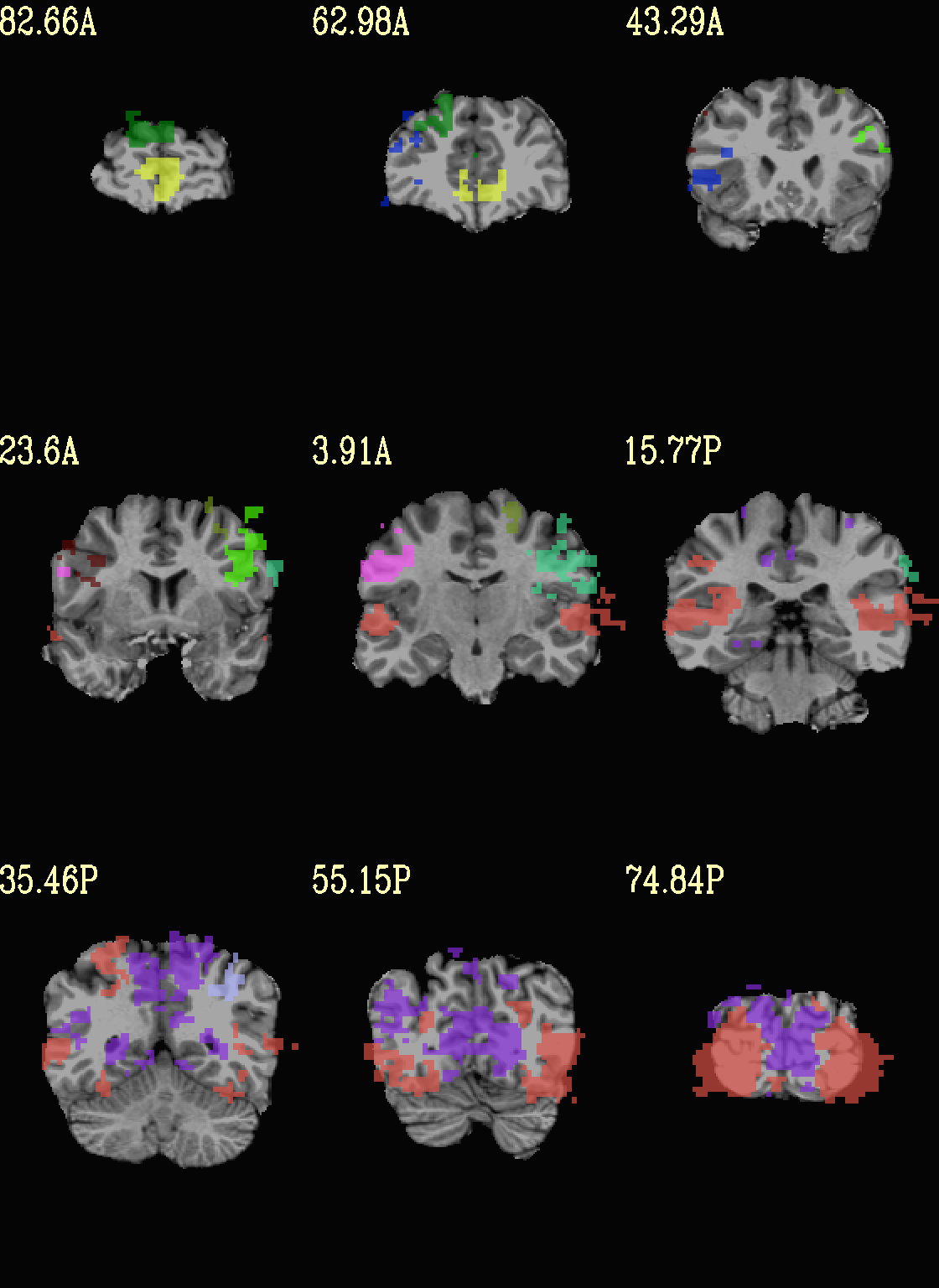
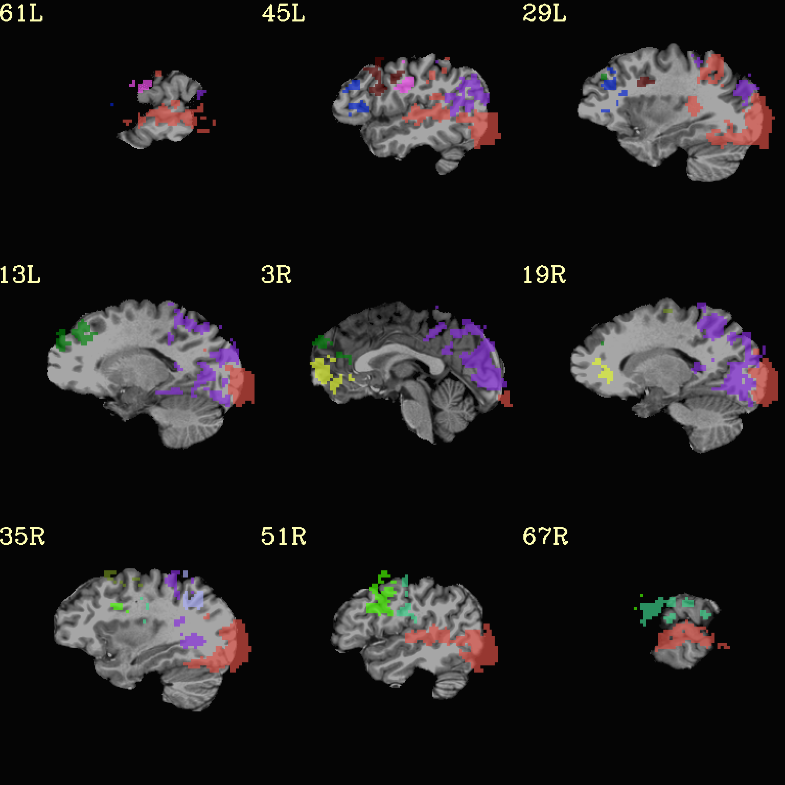
Here we view the cluster map of the clusterized data. Each ROI is
“labelled” in the data by having a different integer volume, and the
colorbar used now could accommodate the visualization of up to 64
clusters (there are other integer-appropriate colorbars that go up
higher). Note how we set -pbar_posonly to have the colorbar start
at 0, and we set the upper value of the func range with -func_range
64, so there is one color per integer value.
set opref = QC/ca006b_Vrel
@chauffeur_afni \
-ulay strip+orig.HEAD \
-box_focus_slices AMASK_FOCUS_ULAY \
-olay clust_Vrel_map.nii.gz \
-ulay_range 0% 130% \
-cbar ROI_i64 \
-func_range 64 \
-pbar_posonly \
-opacity 6 \
-prefix ${opref} \
-set_xhairs OFF \
-montx 3 -monty 3 \
-label_mode 1 -label_size 4
Example 6b |
|
|---|---|
|
|
|
Ex. 7: Overlay beta coefs, threshold+clusterize translucently
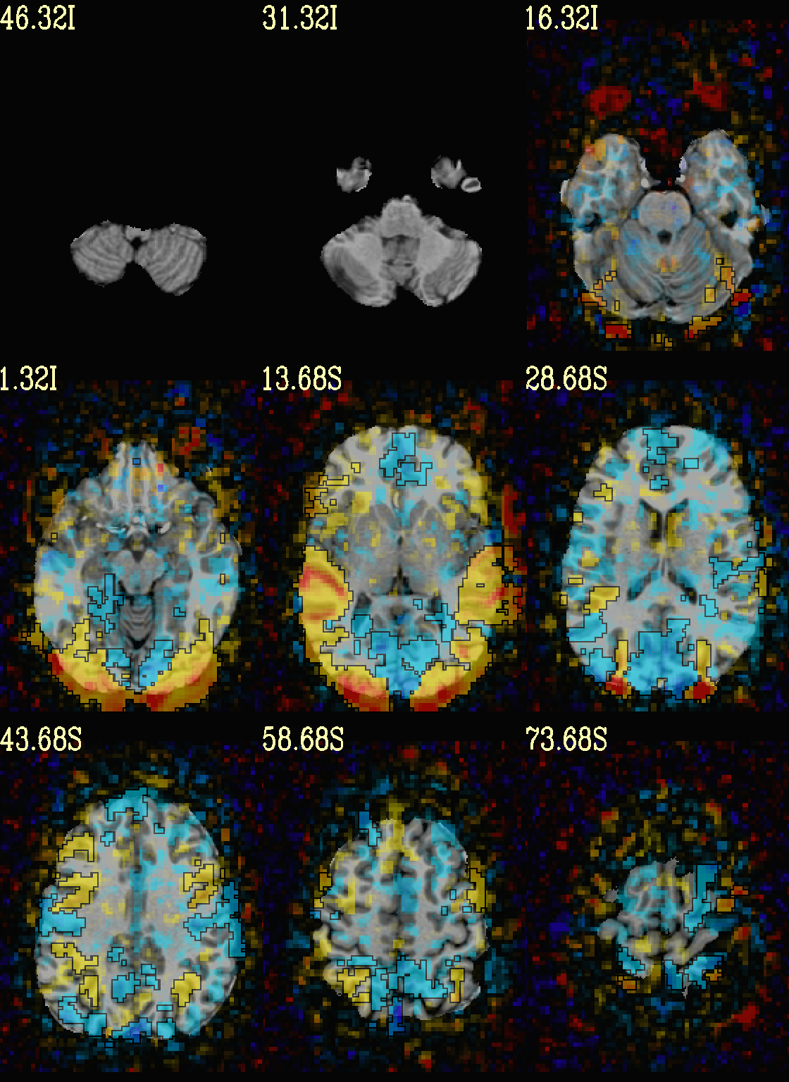
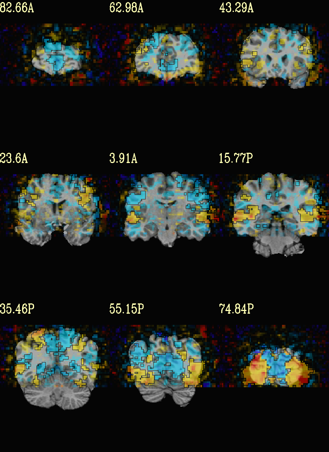
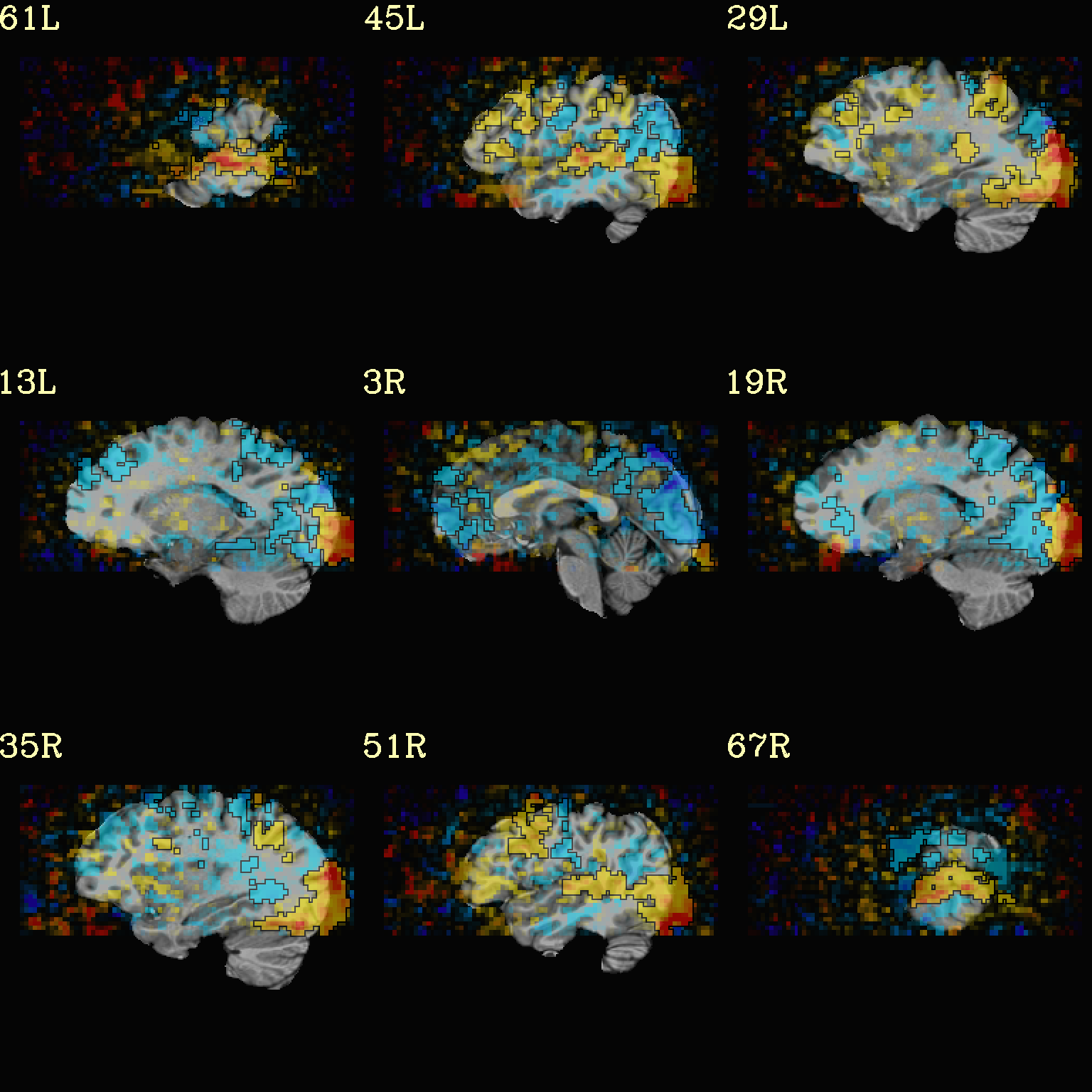
Following on from the previous couple of examples, we can actually apply thresholding (by statistics) and clusterizing with translucent thresholding, using the alpha+boxed methodology from above. This can be a very useful way to highlight some results, while showing more results of modeling.
Therefore:
voxels that are both above voxelwise threshold and in a suprathreshold cluster will be opaque (or at max opacity) and boxed;
voxels that are above voxelwise threshold but not in a large enough cluster will be just slightly translucent and not boxed;
voxels that are below voxelwise threshold (and couldn’t even be in a cluster) will have the usual transparency increasing with their decreasing values.
So, there is a lot happening here. The “trick” with getting this
functionality to work properly is knowing what parameters need to go
where. Which is why we have examples like this! But you might also
want to check out the @chauffeur_afni help.
See how we use -set_subbricks .., -clusterize ..,
-thr_olay_p2stat .. and -thr_olay_pside .. here (and notice
our input for -olay .. is the coefficient+stats dset again, like
we put into 3dClusterize above):
NB: the cluster report text file is also output,
${opref}_clust_rep.txt.
set opref = QC/ca007a_Vrel

@chauffeur_afni                                                       \
    -ulay              strip+orig.HEAD                                \
    -box_focus_slices  AMASK_FOCUS_ULAY                               \
    -olay              func_slim+orig.HEAD                            \
    -cbar              Reds_and_Blues_Inv                             \
    -ulay_range        0% 130%                                        \
    -func_range        3                                              \
    -set_subbricks     -1 "Vrel#0_Coef"  "Vrel#0_Tstat"               \
    -clusterize        "-NN 1 -clust_nvox 200"                        \
    -thr_olay_p2stat   0.001                                          \
    -thr_olay_pside    bisided                                        \
    -olay_alpha        Yes                                            \
    -olay_boxed        Yes                                            \
    -opacity           5                                              \
    -prefix            ${opref}                                       \
    -set_xhairs        OFF                                            \
    -montx 3 -monty 3                                                 \
    -label_mode 1 -label_size 4
Example 7a |
|
|---|---|
|
|
|
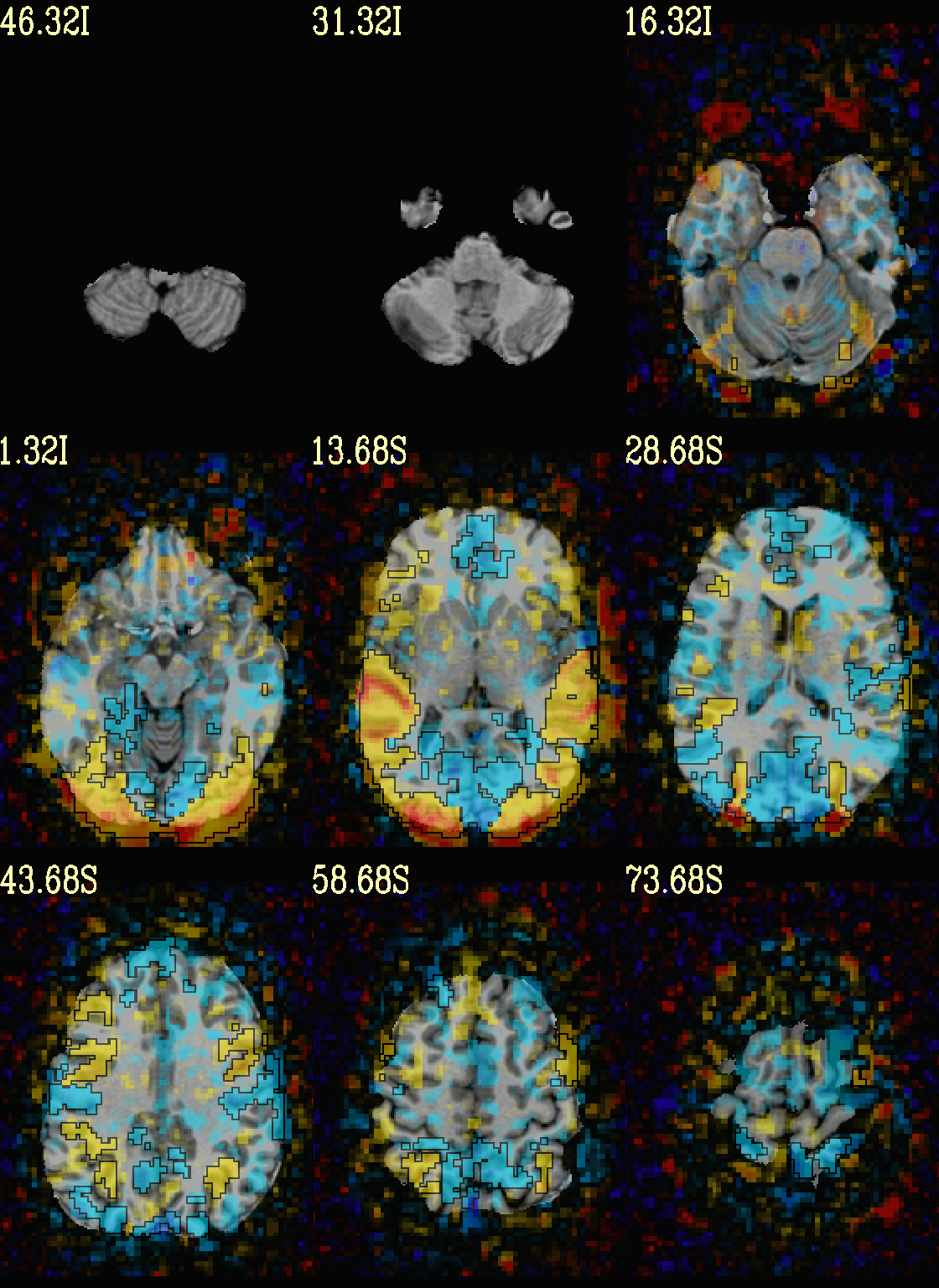
As noted just above, one typically uses a mask when clusterizing (because the cluster size threshold would likely have come from looking at the spatial smoothness of noise just within the brain, not within the entire FOV). That mask can also be included in the commands clusterizing; conveniently, the final images will still show data from the entire FOV, and the boxed voxels will only be within the mask.
The only change from the previous command here is including a -mask
.. option in the chauffeur’s -clusterize .. option, as follows.
Note how the larger clusters that stuck outside the brainmask above
now show the mask’s boundary line—this is particularly apparent in
the posterior part of the brain/FOV.
set opref = QC/ca007b_Vrel_mskd

@chauffeur_afni                                                       \
    -ulay              strip+orig.HEAD                                \
    -box_focus_slices  AMASK_FOCUS_ULAY                               \
    -olay              func_slim+orig.HEAD                            \
    -cbar              Reds_and_Blues_Inv                             \
    -ulay_range        0% 130%                                        \
    -func_range        3                                              \
    -set_subbricks     -1 "Vrel#0_Coef"  "Vrel#0_Tstat"               \
    -clusterize        "-NN 1 -clust_nvox 200 -mask mask.auto.nii.gz" \
    -thr_olay_p2stat   0.001                                          \
    -thr_olay_pside    bisided                                        \
    -olay_alpha        Yes                                            \
    -olay_boxed        Yes                                            \
    -opacity           5                                              \
    -prefix            ${opref}                                       \
    -set_xhairs        OFF                                            \
    -montx 3 -monty 3                                                 \
    -label_mode 1 -label_size 4
Example 7b |
|
|---|---|
|

|

|
Ex. 8: Check alignment with edge view
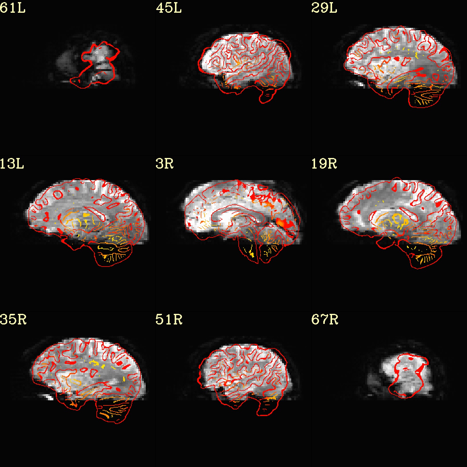
Check out the alignment between two volumes by making and “edge-ified”
version of one and overlaying it on the other. This is quite useful
in many occasions. (Note that this is also the purpose of
@snapshot_volreg, which is also discussed
in this tutorial section here.)
Users can then check the alignment of pertinent things: tissue boundaries, matching structures, etc.
To estimate the edges, we have a particular wrapper, called
@djunct_edgy_align_check. Note that this is mostly an
internally-used convenience script in the afni_proc.py QC, so it
is subject to change (but historically that has just meant adding in
more chauffeur options).
Note that in the present case the EPI hadn’t been aligned to the anatomical yet, so we might not expect great alignment in the present scenario (it’s basically just a question of how much the subject might have moved betwixt scans). The EPI has also relatively low contrast and spatial resolution, so that the lines are fairly course– much more so than if two anatomicals were viewed in this way. There are tricks that one can play to enhance the features of the EPI for such viewing, but that is a larger sidenote (and most readers have likely rightfully given up detailed reading by this point in the webpage).
Because of the general unreliableness of EPI edges, we tend to overlay
the anatomical edges; since the underlay typically determines the
grid, and we don’t want to lose the higher-res info of the anatomical,
we invoke the -use_olay_grid .. option. Some of the inferior
slices look oddly empty of underlay, but that is because this EPI
indeed does not extend that far down.
NB: Since we are edgifying the overlay, we don’t specify the
box-focus dataset by using the AMASK_FOCUS_OLAY option, because
the autoboxing will go awry from the edgification; so we specify the
dataset explicitly.
NB: This wrapper makes JPG images, by default.
set opref = QC/ca008_edgy

@djunct_edgy_align_check                                              \
    -ulay              epi_r1+orig.HEAD"[0]"                          \
    -box_focus_slices  strip+orig.HEAD                                \
    -olay              strip+orig.HEAD                                \
    -use_olay_grid     NN                                             \
    -ulay_range_nz     "2%" "98%"                                     \
    -prefix            ${opref}                                       \
    -montx 3 -monty 3                                                 \
    -label_mode 1
Example 9 |
|
|---|---|

|

|
|
Ex. 10: 4D mode
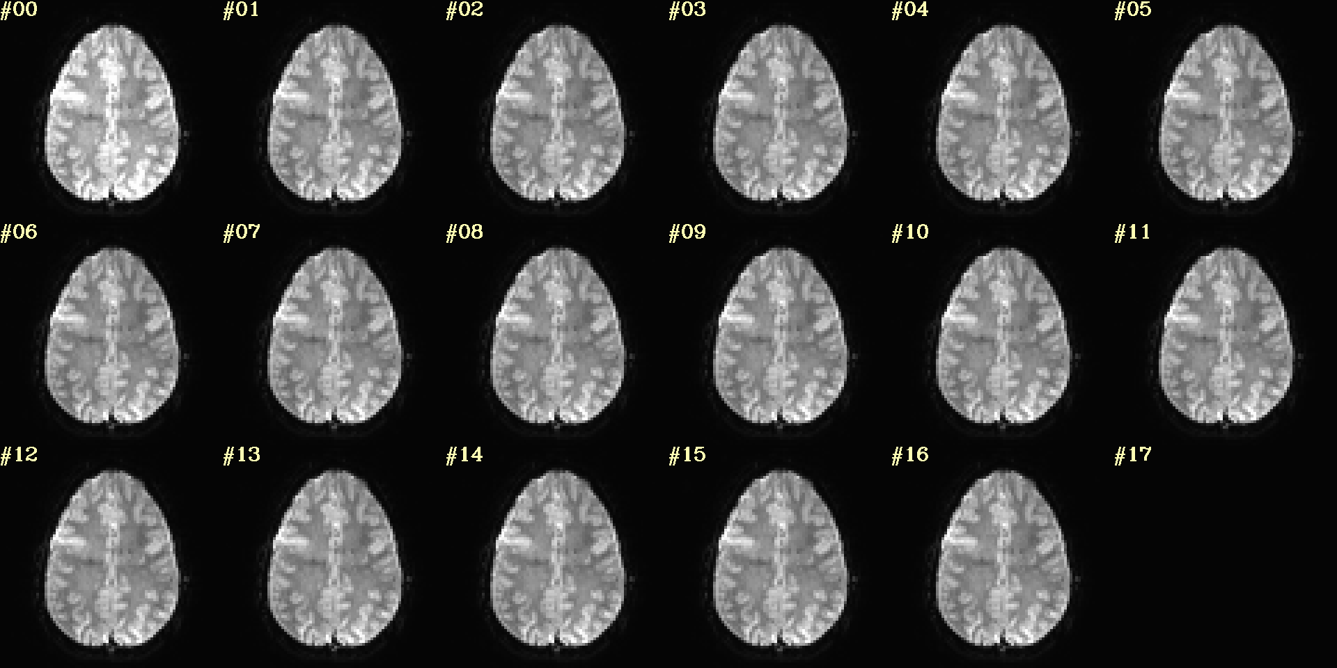
This program can also look at one slice across time, using the
-mode_4Dflag– in the present example, looking at one slice
across the first 17 time points. This might be useful, for example,
to look for distortions across time (e.g., dropout slices, severe
motion or EPI distortion).
By default, a slice is chosen hear the center of the volume’s FOV, but users may specify the location.
Here, the per-slice “xyz” label would not represent the location in
space; instead, we use the -image_label_ijk option to specify
which [n]th volume we are viewing in the time series, starting with
[0].
NB: because this time series is pretty long, we just selected the first 17 volumes of it for display, using subbrick selectors. The program will automatically “guess” something like an appropriate dimensionality for the matrix of images. Weird numbers (primes!!!) might get left with blank spaces, which is fine.
set opref = QC/ca010_epi_4D

@chauffeur_afni                                                       \
    -mode_4D                                                          \
    -image_label_ijk                                                  \
    -ulay          epi_r1+orig.HEAD'[0..16]'                          \
    -prefix        ${opref}                                           \
    -blowup        4                                                  \
    -set_xhairs    OFF                                                \
    -label_mode 1 -label_size 4
Example 10 |
|---|

|
|

|
Ex. 11: Other examples of functionality
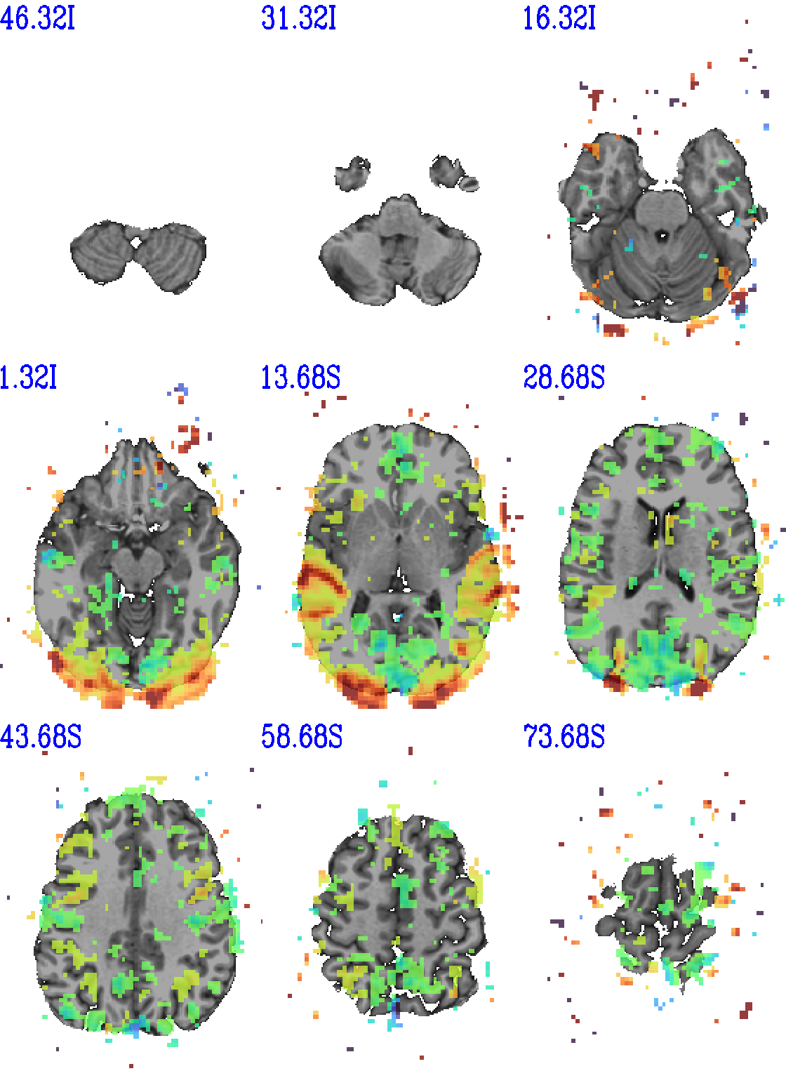
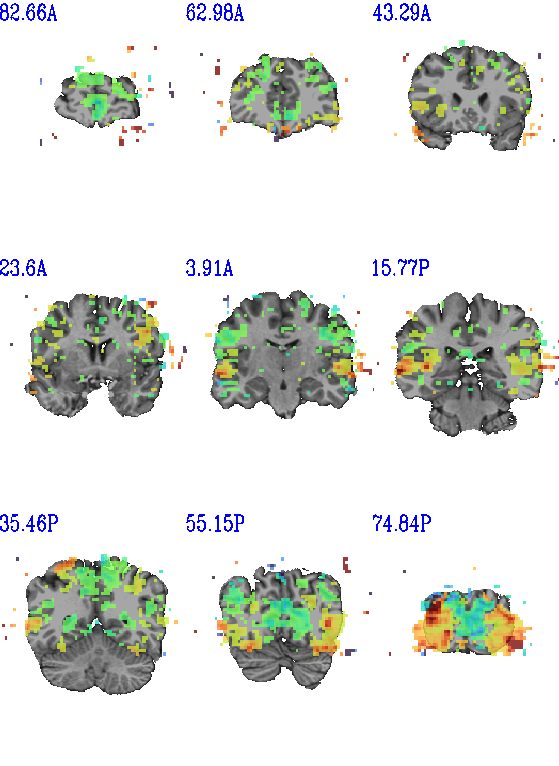
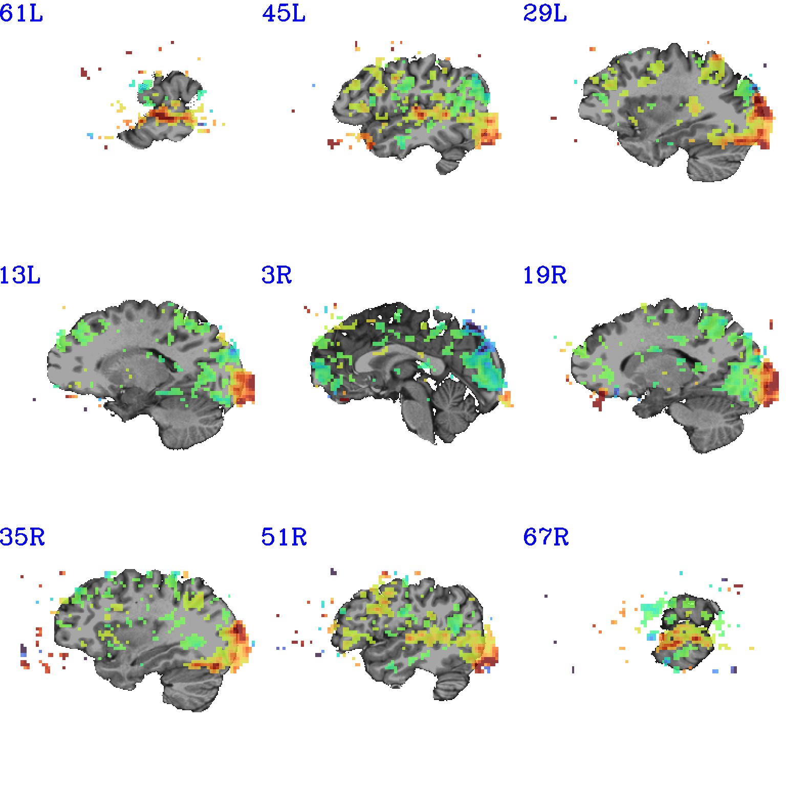
The AFNI GUI can display data in lots of ways. And this wrapper program therefore has lots of options. Here we mention just a couple.
When using an overlay, you can output the colorbar with
-pbar_saveim ... A text file with values describing the range will also be output (same name prefix as the cbar image). You can add comments to this text file, such as what the ranges mean, with-pbar_comm_range ..(this is mainly used by theafni_proc.pyQC generation, but now you know).The background color is controlled with
-zerocolor ...The label text color is controlled with
-label_color ...The resolution at which the images are saved is controlled by the “blowup factor”, which can be controlled with the
-blowup ..option. Larger blowup factors might not affect how the brain images appear, but they will affect how the labels look: higher blowup factors leading to finer labels (which may be harder to read on some screens, depending on settings/programs, though on paper they would look nicer). Larger blowup factors might be necessary for making images to submit as journal figures.You can turn the underlay volume into edges with
-edgy_ulay.You can crop images along any of the three viewing planes, e.g.,
-crop_axi_x CAX1 CAX2will crop an axial image to be between voxels CAX1 and CAX2 along the x-axis (inclusive).You don’t have to output all 3 viewplanes simultaneously. You can turn off outputting, say, the coronal one with
-no_cor.You can control montage features like adding a gap between images, and then putting some color between image panels wtih
-montgap ..and-montcolor .., respectively.There are lots of colorbars to choose from in AFNI; see here.
... and more.
set opref = QC/ca011a_Vrel_coef_stat

@chauffeur_afni                                                       \
    -ulay             strip+orig.HEAD                                 \
    -olay             func_slim+orig.HEAD                             \
    -ulay_range       0% 130%                                         \
    -box_focus_slices AMASK_FOCUS_ULAY                                \
    -func_range       3                                               \
    -cbar             GoogleTurbo                                     \
    -thr_olay_p2stat  0.001                                           \
    -thr_olay_pside   bisided                                         \
    -set_subbricks    -1 "Vrel#0_Coef" "Vrel#0_Tstat"                 \
    -opacity          7                                               \
    -prefix           ${opref}                                        \
    -pbar_saveim      ${opref}                                        \
    -zerocolor        white                                           \
    -label_color      blue                                            \
    -set_xhairs       OFF                                             \
    -montx 3 -monty 3                                                 \
    -label_mode 1 -label_size 4
Example 11a |
|
|---|---|
|
|
|

|
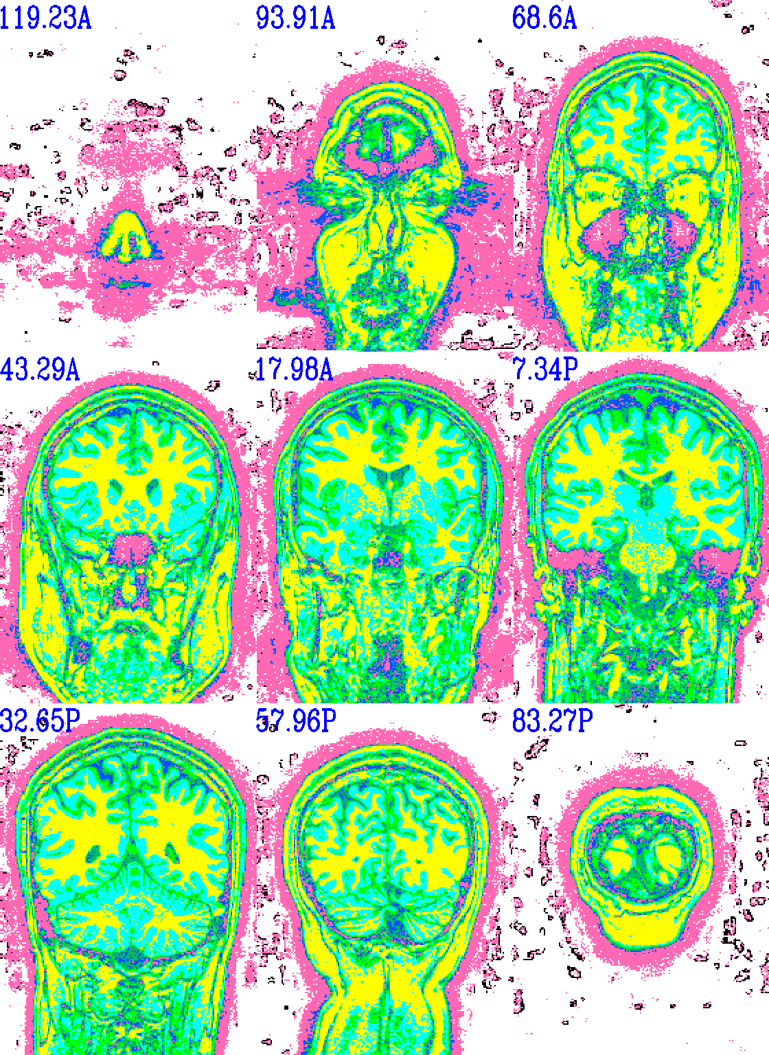
And here is surely a useful example. Well, at least it shows using a specific number of colorblocks for a colorbar, with intervals for each bar specified by the user.
set opref = QC/ca011b_Vrel_coef_stat

@chauffeur_afni                                                       \
    -ulay             anat+orig.HEAD                                  \
    -olay             anat+orig.HEAD                                  \
    -box_focus_slices AMASK_FOCUS_ULAY                                \
    -pbar_posonly                                                     \
    -ulay_range       0% 130%                                         \
    -edgy_ulay                                                        \
    -func_range       1000                                            \
    -cbar_ncolors 6                                                   \
    -cbar_topval ""                                                   \
    -cbar "1000=yellow 800=cyan 600=rbgyr20_10 400=rbgyr20_08 200=rbgyr20_05 100=hotpink 0=none" \
    -opacity          9                                               \
    -prefix           ${opref}                                        \
    -pbar_saveim      ${opref}                                        \
    -zerocolor        white                                           \
    -label_color      blue                                            \
    -set_xhairs       OFF                                             \
    -montx 3 -monty 3                                                 \
    -label_mode 1 -label_size 4
Example 11b |
|
|---|---|

|
|

|

|
Troubleshooting
Occasionally, badness will happen while running @chauffeur_afni.
The most common error I get is about having filenames or paths wrong
(but that might just be me, sadly). Sometimes more insidious or odd
error messages pop up, though. Here are a couple notes on address
some that I have seen.
Many of the issues relate to the fact that this program uses Xvfb
(the “X virtual framebuffer”) to open the AFNI GUI in a virtual
environment. So, in fact, most problems relate to sorting out
something with that underlying program that is called.
On Macs, you might see the following kind of streaming messages in the terminal, and images will not be created:
-- trying to start Xvfb :570
[1] 53344
_XSERVTransmkdir: ERROR: euid != 0,directory /tmp/.X11-unix will not be created.
_XSERVTransSocketUNIXCreateListener: mkdir(/tmp/.X11-unix) failed, errno = 2
_XSERVTransMakeAllCOTSServerListeners: failed to create listener for local
(EE)
Fatal server error:
(EE) Cannot establish any listening sockets - Make sure an X server isn't already running(EE)
I have seen this occur on Mac OS 10.14 and 10.15. From trial-and-error of online solutions, the following has appears to be a good solution (NB: it does require having administrative or
sudoprivileges):mkdir /tmp/.X11-unix sudo chmod 1777 /tmp/.X11-unix sudo chown root /tmp/.X11-unix/
After running that, try executing your
@chauffeur_afnicommand again.One bad thing that can happen on any OS is that if
@chauffeur_afniis interrupted while theXvfbpart is up and running, thenXvfbcan just stay open in the background, ad infinitum. You can see this if you type:ps
in a terminal to display the currently running processes, and the “CMD” column on the right might show “Xvfb”. For example, the output of
psmight look like the following, even when no command appears to be actively running:PID TTY TIME CMD 4963 pts/1 00:00:00 bash 5156 pts/1 00:00:00 Xvfb 5419 pts/1 00:00:00 ps
Sometimes, this scenario can block other
Xvfbjobs from running in the same terminal, effectively blocking you from running@chauffeur_afnior other Xvfb-dependent programs in that terminal.To solve this, you can tell the terminal to stop that specific
Xvfbjob. Take the “PID” (= process ID) for theXvfbjob (in the above case, it is 5156), and use thekillcommand to force it to stop, such as the following here:kill -9 5156You might not need the
-9option, but that let’s the terminal know that you mean business! After that, try your@chauffeur_afnicommand again, and see if things are sorted. Oh, and if you do have to stop anXvfbinstance this way, try not to get the wrong PID, because you might force another job to stop…
